3.3 Hands-on: Value Iteration and Q-Learning

Section goal: Run value iteration and Q-Learning in the same 4×4 GridWorld, observe how the goal reward reaches the starting state, and compare how the two algorithms obtain information.

Learning path: 3.1 State Values and the Bellman Expectation Equation → 3.2 Action Values and the Bellman Optimality Equation → 3.3 Value Iteration and Q-Learning

Code and resources: experiment script · GridWorld diagram · value iteration diagram · Q-Learning curves

3.3.1 Running the GridWorld Experiment

3.1 and 3.2 introduced state values, action values, and Bellman equations. We will now pause the introduction of new equations and place the Bellman optimality equation into a complete small experiment. This allows us to observe a value table as it starts from all zeros and is repeatedly updated until it stabilizes.

The task has only 16 states. The agent starts in the upper-left corner at $S=(0,0)$ and must reach $G=(3,3)$ in the lower-right corner; $X=(1,1)$ is a trap. At each step, the agent can move up, down, left, or right. If it hits a wall, its position does not change.

Figure 3-3: Value iteration and Q-Learning use the same 4×4 GridWorld.

This experiment depends only on the Python standard library and completes within a few seconds on an ordinary computer. Run the following command from the repository root:

python3 code/chapter03_mdp/gridworld_q_learning.py \
  --output-dir output/value-experiment

The script first gives value iteration access to the complete grid rules and repeatedly updates every state. It then lets Q-Learning start from the initial state and update its Q-table using only the experience it actually encounters. After the run, examine three results: how many sweeps value iteration takes to converge, how many sweeps the goal reward takes to reach the starting state, and whether Q-Learning finds the six-step shortest path after exploration is disabled.

3.3.2 Rewards in GridWorld

Entering the goal gives a reward of $+1$, while entering the trap gives a reward of $-1$; both events end the current episode. Every other step gives a reward of $-0.01$. This small negative reward encourages the agent to reach the goal quickly: among successful routes, a six-step route produces a higher return than an eight-step route. We set the discount factor to $\gamma =0.95$.

First, calculate the shortest distance. The row coordinates of the starting state and goal differ by 3, as do their column coordinates, so the agent needs at least

$$|3-0|+|3-0|=6$$

steps.

The trap blocks some routes but does not block every six-step path. The agent can move right three times along the upper boundary and then down three times to reach the goal without encountering the trap. We therefore have an initial criterion for checking the result: if the learned route takes more than six steps, the algorithm has not yet found a shortest path.

Terminal Rewards Are Computed Upon Entry

Before updating the value table, consider the cell $(3,2)$ immediately to the left of the goal. From this cell, one step to the right enters the goal and gives a reward of $+1$:

$$(3,2)\stackrel{\to ,+1}{\to }G\text{terminate}.$$

The episode has ended, so no further actions or rewards follow the goal. The return for moving right from $(3,2)$ is therefore 1:

$$Q((3,2),\to )=1.$$

Written as a Bellman update,

$$Q((3,2),\to )=1+\gamma V(G)=1,$$

where $V(G)=0$. This zero means that no further return is produced after entering the goal; the goal reward has already been counted on the transition into $G$.

The trap is handled in the same way. The transition into $X$ gives a reward of $-1$, after which the episode ends, so $V(X)=0$.

The code returns the reward and termination flag in this temporal order:

def transition(state, action):
    if state in TERMINALS:
        return state, 0.0, True

    next_state = move_or_stay(state, action)
    if next_state == GOAL:
        return next_state, 1.0, True
    if next_state == TRAP:
        return next_state, -1.0, True
    return next_state, -0.01, False

Both value iteration and Q-Learning call this transition function, so they solve the same task.

3.3.3 Value Iteration: Reading the Environment Rules

Value iteration applies when the environment rules are known. Here, "known rules" means that for any cell and any action, we can determine the next cell, the reward, and whether the episode ends.

The algorithm first sets the value of every cell to 0:

$$V_0(s)=0,\forall s.$$

How Far One Sweep Can Propagate Information

Next, the algorithm computes a new value table. For each nonterminal cell, it calculates the values of the four actions—up, down, left, and right—and retains the largest:

$$V_{k+1}(s)=\underset{a}{\max }\left[r+\gamma V_k(s^{\prime })\right].$$

Here, $V_k$ is the old table before the update, and $V_{k+1}$ is the new table produced by this sweep. Computing the entire new table using only the preceding old table is called a synchronous update.

Consider the first sweep. From $(3,2)$, one step to the right enters the goal, giving

$$V_1(3,2)=\underset{a}{\max }\left[r+0.95V_0(s^{\prime })\right]=1.$$

The cell $(2,3)$ above the goal can also enter it in one step, so its value is also 1.

Now consider $(3,1)$, which is two steps from the goal. Although the cell immediately to its right is $(3,2)$, whose value was just computed, the first sweep can read only the old table, where $V_0(3,2)$ is still 0:

$$V_1(3,1)=-0.01+0.95V_0(3,2)=-\mathrm{0.01.}$$

Only in the second sweep can $(3,1)$ read $V_1(3,2)=1$ from the new table:

$$V_2(3,1)=-0.01+0.95V_1(3,2)=\mathrm{0.94.}$$

These two cells illustrate value propagation. The first sweep updates cells one step from the goal, and the second sweep then affects cells two steps away. One synchronous update can propagate the goal reward outward by only one layer.

The implementation performs the same computation. values stores $V_k$, while updated stores the $V_{k+1}$ currently being computed:

values = {state: 0.0 for state in all_states()}

for sweep in range(1000):
    updated = values.copy()
    for state in all_states():
        if state not in TERMINALS:
            updated[state] = max(
                reward if done else reward + GAMMA * values[next_state]
                for action in range(4)
                for next_state, reward, done in [transition(state, action)]
            )
    values = updated

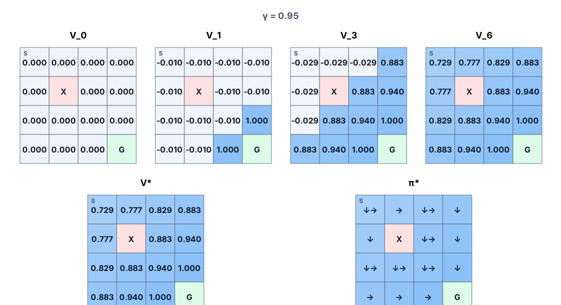
The following figure shows the value tables after sweeps 0, 1, 3, and 6. Begin with the darker blue cells: they appear near the goal and spread gradually toward the upper-left corner as the number of updates increases. In $V_1$, only the two cells adjacent to the goal have positive values. The goal reward reaches the starting state along a six-step path only in $V_6$.

Figure 3-4: Synchronous value iteration. Each sweep uses the complete value table from the preceding sweep.

Reading a Policy from the Value Table

After the sixth sweep, the value table no longer changes. The program computes one more sweep, finds that every cell retains the same value, and stops after sweep 7. This state is called convergence.

The final result is

Row / column	0	1	2	3
0	0.729	0.777	0.829	0.883
1	0.777	0.000 (trap)	0.883	0.940
2	0.829	0.883	0.940	1.000
3	0.883	0.940	1.000	0.000 (goal)

Now check the value of the starting state. Along a shortest path, each of the first five steps gives $-0.01$, and the final step enters the goal and gives $+1$. Discounting these six rewards in order gives

$$\begin{array}{rl}{V}^{\ast }(0,0)& =-0.01-0.95\times 0.01-\cdots -0.95^4\times 0.01+0.95^5\times 1\\ & \approx \mathrm{0.728537.}\end{array}$$

The result is approximately 0.729, matching the value in the upper-left corner of the table. Thus, the starting-state value computed by the program can be verified directly from a concrete shortest path.

Multiple arrows in the figure indicate that a cell has more than one optimal action. From the starting state, for example, moving right first or moving down first can both avoid the trap and reach the goal within six steps.

3.3.4 Q-Learning: Learning from Interaction

Whenever value iteration updates a cell, it can query the results of all four actions directly. Q-Learning does not have this information. It does not know where an action will lead, so it must start at the initial state, select an action, and observe the reward $r$ and next state $s^{\prime }$.

After one step, we obtain an experience tuple $(s,a,r,s^{\prime })$: from state $s$, the agent takes action $a$, receives reward $r$, and enters state $s^{\prime }$. Q-Learning uses this experience to update one Q-value:

$$Q(s,a)\leftarrow Q(s,a)+\alpha \left[r+\gamma \underset{a^{\prime }}{\max }Q(s^{\prime },a^{\prime })-Q(s,a)\right].$$

The first part inside the brackets,

$$r+\gamma \underset{a^{\prime }}{\max }Q(s^{\prime },a^{\prime }),$$

is called the TD target. It combines the reward already received on this step with the currently estimated best value of the next state. The learning rate $\alpha$ determines how far the current update moves toward the TD target.

If $s^{\prime }$ is the goal or trap, the episode has ended, so the next-state value is 0:

next_state, reward, done = transition(state, action)
next_best = 0.0 if done else max(Q[next_state])
td_target = reward + gamma * next_best
Q[state][action] += alpha * (td_target - Q[state][action])

The distinction between the two algorithms is now clear. One sweep of value iteration visits every nonterminal state and compares all four actions in each state. One Q-Learning update uses only the single transition just experienced. Q-Learning must run many episodes before the different state–action pairs have all been updated.

How the Exploration Rate Affects Training Return

At the start of training, every entry in the Q-table is 0, so the agent does not yet know which direction to take. If it always selects an action with the largest current Q-value, many untried routes may never be updated. We therefore use an $\epsilon$-greedy policy: with probability $\epsilon$, the agent selects a random action; with probability $1-\epsilon$, it selects an action with the largest current Q-value.

The experiment uses a learning rate of $\alpha =0.15$ and trains for 500 episodes. To prevent one random run from being unusually good or bad by chance, each setting is run independently with 30 different random seeds.

To plot the curves, we first average the reward at each episode across the 30 runs and then compute a 20-episode moving average. This preserves the overall trend while reducing fluctuations caused by individual random runs.

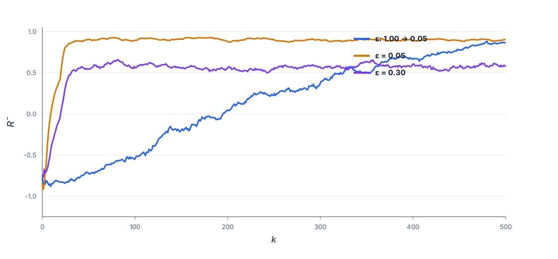
We compare three $\epsilon$-greedy settings:

• $\epsilon$ decreases linearly from $1.00$ to $0.05$;
• fixed $\epsilon =0.05$;
• fixed $\epsilon =0.30$.

Figure 3-5: Training returns under different exploration rates. Each curve aggregates 30 random seeds.

Exploration-rate setting	Mean reward over final 100 episodes	Success rate without exploration	Mean path length
$\epsilon :1.00\to 0.05$	0.803	100%	6.0 steps
Fixed $\epsilon =0.05$	0.900	100%	6.0 steps
Fixed $\epsilon =0.30$	0.563	100%	6.0 steps

With fixed $\epsilon =0.30$, each step still has a 30% probability of selecting a random action. Even after the Q-table has been learned, the agent may take detours or enter the trap during training, so the curve remains at a lower level. This does not necessarily mean that the Q-table has failed to learn a shortest path; exploratory actions may simply have reduced the score in the current episode.

To inspect the learned policy separately, we set $\epsilon =0$ after training. The agent then stops exploring randomly and always selects an action with the largest Q-value. All three settings reach the goal in six steps, with an undiscounted episode reward of

$$5\times (-0.01)+1=\mathrm{0.95.}$$

The training curve records the rewards obtained while the agent is both exploring and acting. Testing with exploration disabled always selects an action with the largest Q-value and therefore evaluates the final policy represented by the Q-table.

A fixed $\epsilon =0.30$ lowers the training return. In this small environment and under the current training budget, all three settings nevertheless learn a shortest path of the same length.

Section Summary

• Value iteration uses a complete environment model and updates every state synchronously. In this section's GridWorld, the goal reward reaches the starting state after six update sweeps.
• No future return follows a terminal state. The terminal reward is received upon entering the goal or trap, and the value of the terminal state is set to 0.
• Q-Learning does not require an environment model. Each interaction produces one transition sample and updates the Q-value of one state–action pair.
• Exploratory actions during training affect episode rewards. Setting $\epsilon$ to 0 for evaluation reveals the greedy policy represented by the Q-table.

The next section, Dynamic Programming, Monte Carlo, and Temporal Difference, begins with this distinction and compares three update methods: complete sweeps, full-episode sampling, and one-step bootstrapping.