3.5 From Q to Q-Learning

Section Preview

Core ideas

• A $V$ table is not enough: without an environment model, knowing whether a situation is “good” does not directly tell you what to do.
• Extend the table by one dimension (a $Q$ table): store a separate score for each “state-action pair”.
• From value to policy (greedy choice): control problems ultimately need a policy $\pi$, not just a score table; the greedy rule turns $Q$ into executable action choices.
• The Bellman optimality equation: the recursion that a perfect optimal $Q$ table must satisfy.
• Q-Learning: take one step, compute a TD target, update one entry.
• Off-policy and exploration: allow yourself to explore randomly while learning, in your head, the most rational way to act.

In the previous section, we introduced three value-estimation methods: DP, MC, and TD. Their shared goal is to estimate a state-value table $V(s)$: one number per state, representing how much return we can expect, on average, if we continue from here.

This table is already a big step beyond staring at immediate rewards. It no longer asks “how many points do I get this step?”, but “starting from this situation, how many points is it worth in the long run?”. However, for control, we are still missing the last step: an agent must ultimately choose actions. Knowing only how valuable a state is overall does not necessarily tell us whether, in that state, we should go left, go right, jump, or stop.

Let’s look at a concrete scene. Suppose the current CartPole state has a high value. That statement means “if we act appropriately from now on, the pole will likely remain balanced for a long time.” But it does not say whether we should push left or push right right now. To answer that, we need to compare:

• In the same state $s$, if we take action $a_1$ first and then continue under some policy, what is the expected return?
• If we take another action $a_2$ first and then continue, what is the expected return then?

In other words, state value answers “is this situation good or bad?”, while control needs “in this situation, which actions are good or bad?”. This is exactly the role of the action-value function $Q(s,a)$.

If the environment model is known, we can derive action values from $V^\pi$. Given a policy $\pi$, if we take action $a$ in state $s$, we obtain an immediate reward $R(s,a)$, and then transition to the next state $s'$ with probability $P(s'\mid s,a)$. From $s'$ onward, the future value is captured by $V^\pi(s')$. Therefore:

$$Q^\pi(s,a) = R(s,a) + \gamma \sum_{s'} P(s'|s,a) \, V^\pi(s'),$$

The meaning is straightforward: the action value equals “the immediate reward from taking this action”, plus “the discounted expected value of the next state induced by this action”. The real problem is that, in practical tasks, we typically do not know $R$ and $P$. The agent cannot see the full transition table, nor the expected reward of each action; it can only try actions repeatedly, observe the actual reward $r$, and see the actual next state $s'$.

So a natural idea appears: since, under an unknown model, it is hard to compute $Q$ using $P$ and $R$, why not do what we did for $V(s)$ and learn the value of each state-action pair directly? We extend the table from “one cell per state” to “one cell per action under each state”. This table is the action-value table, i.e., the $Q$ table.

Once we have $Q(s,a)$, a policy can be obtained directly by choosing the action with the largest action value at each state:

$$\pi(s) = \operatorname*{arg\,max}_a Q(s,a).$$

Key Concept

First, separate two names: $Q(s,a)$ and Q-Learning.

$Q(s,a)$ is the action-value function. In tabular problems, you can view it as an action-value table. Unlike $V(s)$ (one number per state), $Q(s,a)$ stores one number for each action at each state. So $Q(s,a)$ does not answer “is this state good?”, but rather “in this state, if I take this action first and then continue acting, how good is the long-run outcome?”.

In the classic paper, Q-Learning (Watkins & Dayan, 1992) is defined as a model-free, off-policy TD control algorithm. It updates $Q(s,a)$ from one-step experience, using $\max_{a'} Q(s',a')$ as an estimate of the “optimal action value” at the next state, and thereby iteratively approaches the optimal action-value function $Q^*$.^[1][2]

In the tabular setting, Q-Learning’s goal is simply to learn this $Q$ table accurately. Each time it collects a transition $(s,a,r,s')$, it constructs a learning target of the form “immediate reward + max $Q$ in the next state”. After learning, in each state, choosing the action with the largest $Q$ value yields the policy induced by the action-value table.

Key formulas

$$Q^\pi(s,a)=\mathbb{E}_\pi[G_t\mid S_t=s,A_t=a] \quad \text{(Action value: fix the first action, then evaluate the future return)}$$

$$Q^*(s,a) = \mathbb{E}\left[ r+\gamma\max_{a'}Q^*(s',a') \mid s,a \right] \quad \text{(Bellman optimality equation: the self-consistency an optimal $Q$ must satisfy)}$$

$$Q(s,a) \leftarrow Q(s,a) + \alpha\left[ r+\gamma\max_{a'}Q(s',a')-Q(s,a) \right] \quad \text{(Q-Learning update: correct one action value using one interaction)}$$

The logic chain across the three lines:

• Line 1 defines what $Q(s,a)$ means: in state $s$, take action $a$ first, then follow policy $\pi$; $Q$ is the expected return.
• Line 2 states the target: for the optimal action values, “from the next state onward, act optimally”, which leads to the $\max$.
• Line 3 gives the algorithm: use one sample transition to build a TD target, then move the current estimate toward it by a learning rate $\alpha$.

Before we go further, let’s use an example to make the new object $Q(s,a)$ feel necessary.

Why Do We Need $Q(s,a)$ If We Already Have $V(s)$?

The real issue is this: in control, we do not just want to evaluate a situation; we must decide an action. A state-value function $V^\pi(s)$ can tell you “how good it is to be in $s$ under policy $\pi$”, but it does not tell you, inside $s$, which action is better.

Look at it from another angle. Suppose we are in the same state $s$ and we have two candidate actions $a_1$ and $a_2$. To decide, what we truly need is the comparison:

$$Q^\pi(s,a_1) \quad \text{vs.} \quad Q^\pi(s,a_2).$$

That is, we want to score actions, not just states.

This becomes especially clear when the environment model is unknown. If we knew $P$ and $R$, we might be able to compute $Q^\pi$ from $V^\pi$ as shown earlier. But in most RL settings, the agent learns purely from sampled experience, so learning $Q$ directly is the more natural route.

From $Q$ to a Policy (Greedy Choice)

Once we have $Q(s,a)$, a policy can be derived immediately:

$$\pi(s) = \operatorname*{arg\,max}_a Q(s,a).$$

This simply says: at state $s$, look at the $Q$ values for all actions, and pick the largest. In other words, $Q(s,a)$ scores actions, and $\arg\max$ turns those scores into a concrete choice. The action-value table is therefore not only an evaluation tool; it can directly induce a policy.

This “always pick the action with the highest score” rule is called a greedy policy. We introduce it first not because it is the only possible policy, but because it is the most direct: if $Q(s,a)$ already assigns a score to each action, the most natural behavior is to pick the highest-scoring one.

Of course, in practice, a policy does not have to be defined this way. During training, to explore actions that have not been tried enough, we often add randomness on top of greedy choice. But from the standpoint of “how do we turn $Q$ values into action selection”, greedy choice is the clearest starting point.

Mathematical definition

To define it precisely, the action-value function under policy $\pi$ is:

$$Q^\pi(s,a) = \mathbb{E}_\pi \bigl[G_t \mid S_t=s, A_t=a\bigr] = \mathbb{E}_\pi \bigl[R_{t+1} + \gamma R_{t+2} + \gamma^2 R_{t+3} + \cdots \mid S_t=s, A_t=a\bigr].$$

The condition $S_t=s, A_t=a$ means: we fix the starting state and the first action. Therefore, $Q^\pi(s,a)$ means: in state $s$, take action $a$ first; then, from the next step onward, follow policy $\pi$; what is the expected future return? Written out, that future return is:

$$R_{t+1} + \gamma R_{t+2} + \gamma^2 R_{t+3} + \cdots .$$

The Bellman Optimality Equation

After defining $Q^\pi(s,a)$, we still need to answer a stronger question: if our goal is not to evaluate a fixed policy, but to find the optimal policy, what relationship must the optimal action-value table satisfy?

Let’s return to the intuition. The optimal action value $Q^*(s,a)$ means: in state $s$, take action $a$ first; then, from the next step onward, behave optimally; what is the expected return? Since the first action is fixed, we cannot change it anymore. The real “optimal choice” begins after we arrive at the next state $s'$. Once at $s'$, if we already possess the correct optimal $Q$ table, we should choose the action that maximizes $Q^*(s',a')$.

Therefore, $Q^*(s,a)$ must satisfy the following recursion:

$$Q^*(s,a) = \mathbb{E}\left[ r + \gamma \max_{a'} Q^*(s',a') \mid s,a \right].$$

This is the Bellman optimality equation for $Q$. The right-hand side has two parts:

• $r$ is the immediate reward observed after taking the current action;
• $\gamma\max_{a'}Q^*(s',a')$ is the optimal future value from the next state, discounted by $\gamma$ back to the current time.

This recursion reveals what drives Q-Learning: a correct optimal $Q$ table must be self-consistent. An entry $Q^*(s,a)$ should equal the expected result of “take one step from this entry, then consult the best entry in the next state”. If the current table violates this relationship, the table is not yet correct; the larger the violation, the clearer the update direction.

Q-Learning’s goal is to approximate the solution of this self-consistency equation by repeatedly sampling experience, without knowing the full environment model.

The Q-Learning Update Rule

The Bellman optimality equation gives us a target, but it still contains an expectation. If the model were known, we could average over all possible next states $s'$ and reward branches. In the typical Q-Learning setting, however, the model is unknown. What the agent actually gets is a one-step transition:

$$(s,a,r,s').$$

This is only a single sample, but it provides a local clue: the current estimate $Q(s,a)$ should move toward “the reward we just saw + the best action value we currently believe is available at the next state”. So we use the current $Q$ table to build a sampled Bellman target:

$$\text{target} = r + \gamma \max_{a'} Q(s',a').$$

Two points are worth noticing. First, the target uses only the actually observed one-step transition $(r,s')$, so we do not need the full transition probabilities $P(s'\mid s,a)$. Second, the term $\max_{a'}Q(s',a')$ still comes from the current $Q$ table, which is not yet accurate. This practice of “using an existing estimate to form the next learning target” is called bootstrapping.

Now we have an old estimate and a new target. Their difference is the TD error in Q-Learning:

$$\delta = \text{target} - Q(s,a).$$

If $\delta>0$, this experience suggests that $Q(s,a)$ was underestimated, so we should increase it; if $\delta<0$, the current estimate was overly optimistic, so we should decrease it. The learning rate $\alpha$ controls the correction magnitude, yielding:

$$Q(s,a) \leftarrow Q(s,a) + \alpha \delta.$$

Substituting the target and the TD error gives the standard Q-Learning update:

$$Q(s,a) \leftarrow Q(s,a) + \alpha\left[ r + \gamma \max_{a'} Q(s',a') - Q(s,a) \right].$$

You can read this formula as a compressed version of a three-step process:

1. Take one step and obtain experience $(s,a,r,s')$.
2. Use $r+\gamma\max_{a'}Q(s',a')$ to estimate “what this entry should be now”.
3. Do not overwrite the old value in one shot; move a small step toward the target according to $\alpha$.

Compared with the TD update from the previous section,

$$V(s) \leftarrow V(s) + \alpha[r + \gamma V(s') - V(s)],$$

the change in Q-Learning is not merely replacing $V$ with $Q$. More importantly, the $V(s')$ in the target becomes $\max_{a'}Q(s',a')$. This means that, during updates, Q-Learning always interprets the next state as “from there onward, choose the best-looking action according to the current table”. It is not faithfully evaluating the exploratory behavior policy that is generating data; rather, it uses exploration to collect experience while learning an action-value table that points toward the greedy optimal policy.

GridWorld: From a Numerical Example to Code

Consider a 4×4 GridWorld. Each step gives reward $-1$, the discount factor is $\gamma=0.9$, and the $Q$ table is initialized to all zeros. The agent starts at $(0,0)$, moves right, reaches $(0,1)$, and receives $r=-1$.

In Gymnasium, FrozenLake-v1 is also a 4×4 grid environment. The figure below shows an example run:

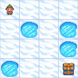
Source: Gymnasium Documentation - Frozen Lake

Let’s see what actually happens in this step. The agent stands at $(0,0)$, chooses “right”, and moves to $(0,1)$. The environment tells it: the reward for this step is $-1$. Therefore, this update will modify only one number: the action value $Q((0,0), \text{right})$. It will not modify the “up/down/left” scores at $(0,0)$, nor any action values in other states.

Now the question becomes: what number should we record for this action? Q-Learning’s idea is to look at what we got now, and then look at what we might get from the next cell. At the very beginning the $Q$ table is all zeros, so in the next state $(0,1)$, no matter which action we choose, the current estimate is still 0:

$$\max_{a'}Q((0,1), a') = 0$$

So the target we see this time is:

$$\text{target} = -1 + 0.9 \times 0 = -1$$

The meaning is simple: this step already costs 1 point, and the next cell does not look good or bad yet, so we treat “go right” as worth $-1$ for now.

But Q-Learning does not immediately replace the old value 0 with $-1$. It moves only a small step toward the target. If the learning rate is $\alpha=0.1$, the update becomes:

$$Q((0,0), \text{right}) = 0 + 0.1 \times (-1 - 0) = -0.1$$

That is, after the first trial, the table only records a mild lesson: from $(0,0)$, going right currently looks a bit worse than before. A single update is small; but with repeated sampling, the $Q$ values along bad (negative-reward) paths keep decreasing, while the $Q$ values along the optimal path gradually increase. Information about the optimal policy propagates backward from the goal to the start, and eventually fills the entire $Q$ table.

Code Implementation

Below is a minimal Q-Learning core implementation that does not rely on external RL libraries.

import numpy as np

rng = np.random.default_rng(0)

N = 4
START = (0, 0)
GOAL = (3, 3)
ACTIONS = [(-1, 0), (0, 1), (1, 0), (0, -1)]  # up, right, down, left
ARROWS = np.array(["↑", "→", "↓", "←"])

def to_state(pos):
    return pos[0] * N + pos[1]

def to_pos(state):
    return divmod(state, N)

def step(state, action):
    row, col = to_pos(state)
    if (row, col) == GOAL:
        return state, 0, True

    dr, dc = ACTIONS[action]
    next_row = min(max(row + dr, 0), N - 1)
    next_col = min(max(col + dc, 0), N - 1)
    next_state = to_state((next_row, next_col))
    done = (next_row, next_col) == GOAL
    return next_state, -1, done

Q = np.zeros((N * N, len(ACTIONS)))
alpha = 0.1
gamma = 0.9
epsilon0 = 0.3

for episode in range(2000):
    state = to_state(START)
    # decay exploration rate over time
    epsilon = max(0.02, epsilon0 * (0.995**episode))

    for _ in range(100):
        # 1. Select an action (exploration vs exploitation)
        if rng.random() < epsilon:
            action = int(rng.integers(len(ACTIONS)))
        else:
            best_actions = np.flatnonzero(Q[state] == Q[state].max())
            action = int(rng.choice(best_actions))

        # 2. Interact with the environment
        next_state, reward, done = step(state, action)

        # 3. Compute TD target and update the Q-table
        bootstrap = 0 if done else Q[next_state].max()
        target = reward + gamma * bootstrap
        Q[state, action] += alpha * (target - Q[state, action])

        state = next_state
        if done:
            break

print("Q-values of the four actions at the start state:")
print(dict(zip(ARROWS, Q[to_state(START)].round(3))))

print(\"\\nOne greedy policy learned:\")
for row in range(N):
    cells = []
    for col in range(N):
        if (row, col) == GOAL:
            cells.append("G")
        else:
            state = to_state((row, col))
            cells.append(ARROWS[int(Q[state].argmax())])
    print(" ".join(cells))

Run output:

Q-values of the four actions at the start state:
{'↑': -5.1, '→': -4.6, '↓': -4.6, '←': -5.2}

One greedy policy learned:
→ → → ↓
↑ ↑ → ↓
↑ ↑ → ↓
↑ ↑ → G

For example, at the start state, the learned $Q$ values for the four actions are: up $-5.1$, right $-4.6$, down $-4.6$, left $-5.2$. This indicates that, in terms of long-run return, “right” and “down” are both better than “up” and “left”.

Off-Policy, Exploration, and the CliffWalking Example

So far we have focused on the update rule itself. But the more subtle question is: when the agent is exploring, what policy is it actually learning about?

To see the difference, consider CliffWalking, the standard example in Sutton & Barto and a built-in environment in Gymnasium.

The environment is a 4-row × 12-column grid. The agent starts from S at the bottom-left and aims to reach G at the bottom-right. Each step can move one cell up, down, left, or right.

Rule	Description
Start	bottom-left S (row 4, col 1)
Goal	bottom-right G (row 4, col 12)
Normal step	reward $-1$
Fall off cliff	reward $-100$, immediately return to start S; episode continues
Hit a wall	stay in place, reward $-1$
Termination	episode ends when reaching G

The shortest path from S to G hugs the cliff edge and takes 11 steps. But it is dangerous: during exploration, if the agent happens to step down by mistake, it falls off the cliff and loses 100 points.

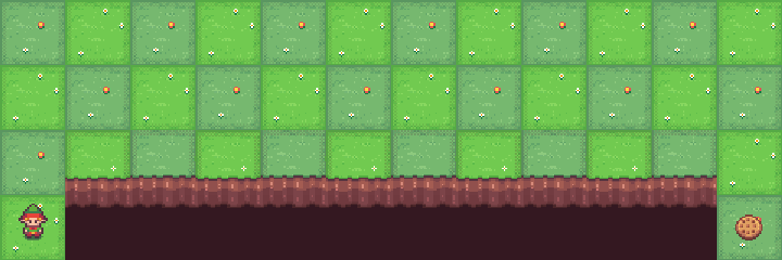
Source: Gymnasium Documentation - Cliff Walking. The original environment is adapted from Sutton and Barto, Reinforcement Learning: An Introduction, Example 6.6.

Q-Learning (off-policy) uses $\max_{a'} Q(s',a')$ in its target, which assumes that the future always takes the optimal action. Therefore it learns the shortest cliff-hugging path.

SARSA (on-policy) uses the target $r + \gamma Q(s', a')$, where $a'$ is the action actually sampled from the current behavior policy (typically $\varepsilon$-greedy). Since SARSA accounts for the risk of exploration-induced mistakes inside its update, it tends to learn a safer path away from the cliff, even if it is longer.

The difference between the two algorithms comes from different assumptions about “the future policy”:

• Q-Learning estimates the value of the optimal policy, independent of how the current behavior policy explores.
• SARSA estimates the value of the current behavior policy, so it avoids risks introduced by exploration.

This is not a question of which one is “better”. They answer different questions. Q-Learning answers “if we ignore the randomness of exploration, what is the ideal optimum?” SARSA answers “given the exploration noise we are actually using, what is the safest way to behave?”.

Limitations of Tabular Methods

At this point, Q-Learning seems to have solved decision-making under an unknown model: no environment model is needed, we do not have to wait until the end of an episode, and we can update after every step. The convergence behavior on 4×4 GridWorld supports this.

But it relies on a fundamental assumption: the numbers of states and actions must be small enough to fit in a table.

In 4×4 GridWorld, we have only 16 states × 4 actions = 64 $Q$ values. But in robot control, the state may include countless combinations of angles and velocities, forming a continuous space with infinitely many states. In video games, the state may be an image frame, and the number of possible pixel configurations is far beyond what any table can store. A table simply cannot fit.

So the core idea of Q-Learning has not become obsolete: iteratively approximate the solution to the Bellman optimality equation using TD targets. What becomes infeasible is “store a separate row for every state-action pair”. Chapter 4 will tackle this exact issue: if a table cannot fit, can we use a neural network to approximate the entire $Q$ function? The answer is Deep Q-Networks (DQN).

Previous section: DP, MC, and TD | Next section: From Value to Policy

Summary

• The action-value function $Q(s,a)$ assigns a value estimate to each state-action pair. For decision-making, we can directly choose the action with the largest $Q$ value, without an environment model.
• Q-Learning updates the $Q$ table using the TD target $r+\gamma\max_{a'}Q(s',a')$, and gradually approaches the solution of the Bellman optimality equation through bootstrapping.
• An $\varepsilon$-greedy policy explores randomly with probability $\varepsilon$ and exploits the currently best action with probability $1-\varepsilon$, balancing exploration and exploitation.
• Off-policy: Q-Learning separates the behavior policy ($\varepsilon$-greedy) from the target policy (greedy), allowing it to learn the optimal policy while exploring.
• Once the state space grows large, tabular methods break down and we must introduce function approximation (deep reinforcement learning).

Exercises

1. In the 4×4 GridWorld, if $\gamma=1$, what is the return of the shortest path? If it takes 8 steps to reach the goal, what is the return then?
2. If we change the reward to “+10 upon reaching the goal, 0 for each step”, will the agent still prefer the shortest path? Why?
3. In the Q-Learning update, what kind of policy tendency would we get if we replace $\max_{a'}Q(s',a')$ with the average over all actions?
4. Why can Q-Learning learn from old experience, while SARSA depends more on new experience generated by the current policy?

References

---

1. Watkins, C. J. C. H., & Dayan, P. (1992). Q-learning. Machine Learning, 8(3-4), 279-292. DOI: https://doi.org/10.1007/BF00992698；Author page: https://www.gatsby.ucl.ac.uk/~dayan/papers/wd92.html. ↩︎

2. Sutton, R. S., & Barto, A. G. (2018). Reinforcement Learning: An Introduction (2nd ed.). MIT Press. ↩︎