3.3 V(s): Value Functions and Bellman Equations

Section Guide

Core content

• $V^\pi(s)$: evaluates how much future return policy $\pi$ can obtain on average from state $s$.
• Bellman equation: rewrites “looking through the whole future” as “immediate reward + next-state value”.
• Value table: in finite-state problems, stores each state’s $V(s)$ as a set of numbers that can be updated.
• From $V$ to $Q$: first evaluate a policy, then compare actions, and finally use that comparison to find a better policy.

In the previous section, we built the formal framework of RL: an MDP describes the environment rules, $G_t$ measures the total return of a trajectory, and a policy $\pi$ specifies how actions are chosen at each step. With these symbols, we can already describe how an agent interacts with an environment. But description is not solution. Reinforcement learning ultimately cares about the policy: in the same state, changing the action-selection rule can lead to a completely different future. Therefore, before discussing “how to find a good policy,” we first need to solve a basic problem that serves policy improvement: how do we evaluate the current policy’s performance in each state?

The state-value function $V^\pi(s)$ is prepared for exactly this problem. It asks: if the agent is currently standing in state $s$, and from this moment onward always acts according to policy $\pi$, how much total return can it obtain on average in the future? Notice that $V^\pi(s)$ is not a score that naturally belongs to the state itself. It is the performance of policy $\pi$ in state $s$. In the same CartPole situation, a bad policy may quickly let the pole fall, while a good policy can keep it balanced. The state is the same; the policy is different; therefore the value is different.

Directly computing $V^\pi(s)$ seems to require enumerating every possible future trajectory starting from $s$, which is usually impossible. The role of the Bellman equation is to break this long-term evaluation into a one-step recursion: first look at the immediate reward, then delegate the remaining future to the value of the next state. In this way, policy evaluation no longer needs to see the entire future at once. It can gradually propagate information backward through relationships between neighboring states.

Given a policy $\pi$, how do we evaluate its performance in every state? Further, if we want a better policy, how do we move from “evaluating states” to “choosing actions”?

Core concept

The Bellman equation connects “policy evaluation” and “policy improvement”: first use $V^\pi$ to evaluate a policy, then use $Q$ or an optimality equation to compare actions, so the policy has a direction for improvement.

Core formulas

$$V^\pi(s)=\mathbb{E}_\pi\left[\sum_{k=0}^{\infty}\gamma^k r_{t+k}\mid s_t=s\right] \quad \text{(definition of state-value function: evaluates the long-term return of policy $\pi$ in state $s$)}$$

$$V^\pi(s)=\sum_{a\in\mathcal{A}}\pi(a\mid s)\left[R(s,a)+\gamma\sum_{s'\in\mathcal{S}}P(s'\mid s,a)V^\pi(s')\right] \quad \text{(Bellman expectation equation: recursively computes value under a fixed policy)}$$

$$V^*(s)=\max_a\left[R(s,a)+\gamma\sum_{s'\in\mathcal{S}}P(s'\mid s,a)V^*(s')\right] \quad \text{(Bellman optimality equation: defines the optimal state value)}$$

State Value and Bellman Equation:

• $V^\pi(s)$: the value of policy $\pi$ in state $s$, that is, the average total score obtained by starting from $s$ and following policy $\pi$.
• $r_{t+k}$: the one-step reward obtained at future step $k$.
• $\gamma$: the discount factor (Gamma), which controls how much future rewards matter ($0 \sim 1$).
• $\mathcal{A}$: the action space, the set of all actions available in the task. In CartPole, for example, these are usually “push left” and “push right”.
• $\pi(a\mid s)$: the policy, the probability of choosing action $a$ in state $s$.
• $P(s'\mid s,a)$: the state transition probability, the probability of moving to next state $s'$ after taking action $a$ in state $s$.

This section repeatedly uses the following symbols. Let us first make clear what each one means:

Symbol	How to understand it first
$s_t$	The state at step $t$, such as a board position or robot pose
$a_t$	The action at step $t$, such as moving left or outputting a control value
$\mathcal{A}$	The action space, the set of all available actions
$r_t$	The immediate reward obtained at step $t$
$\pi(a\mid s)$	The probability that the policy chooses action $a$ in state $s$
$\gamma$	The discount factor; farther rewards receive smaller weights
$G_t$	The total return accumulated from step $t$ onward
$V^\pi(s)$	The average total return from starting in state $s$ and following policy $\pi$

There is an important distinction here:

• $r_t$ is the immediate reward of the current step. It only looks at one step, and we know it after taking that step.
• $G_t$ is the discounted total return actually obtained along one concrete trajectory starting from step $t$. It looks at a whole trajectory, so different trajectories can have different $G_t$.
• $V^\pi(s)$ is not the score of one trajectory. It is the average of $G_t$ over many possible trajectories that start from state $s$ and then follow policy $\pi$.

What is the difference between G and V? A numerical example

Start with the full definition. The original formula for discounted return $G_t$ is:

$$G_t = \sum_{k=0}^{\infty}\gamma^k r_{t+k}$$

Expanding the summation gives:

$$G_t = r_t+\gamma r_{t+1}+\gamma^2 r_{t+2} +\gamma^3 r_{t+3} +\cdots$$

For demonstration, suppose the discount factor is $\gamma=0.9$. Starting from the same state $s$, we play twice under the same policy, and in each run only keep the first three rewards. In other words, first look at this three-step truncated version:

$$G_t = r_t+\gamma r_{t+1}+\gamma^2r_{t+2}$$

The first run goes smoothly, with three rewards $2,4,6$. Substitute them into the formula:

$$G_t^{(1)} = \underbrace{2}_{r_t} + 0.9\times \underbrace{4}_{r_{t+1}} + 0.9^2\times \underbrace{6}_{r_{t+2}}$$

The result is:

$$G_t^{(1)} = 10.46$$

The second run encounters a bad outcome later, with three rewards $2,1,-3$. Substituting again:

$$G_t^{(2)} = \underbrace{2}_{r_t} + 0.9\times \underbrace{1}_{r_{t+1}} + 0.9^2\times \underbrace{(-3)}_{r_{t+2}}$$

The result is:

$$G_t^{(2)} = 0.47$$

Notice that both runs have the same first-step immediate reward, $r_t=2$, but what happens afterward is different, so the trajectory-level $G_t$ differs greatly. The state value $V^\pi(s)$ is the expectation of these possible $G_t$ values. If we currently only have these two samples, we can use their average as a rough estimate:

$$V^\pi(s)\approx \frac{10.46+0.47}{2}=5.465$$

So $r_t$ is a one-step score, $G_t$ is the total score actually obtained along one trajectory from a certain moment onward, and $V^\pi(s)$ answers: if we start many times from the same state $s$, what is the long-run average of those total scores?

State-Value Function: Evaluating a State

In the previous section, we had the MDP tuple to describe the rules of the game, $G_t$ to measure the total score obtained from a certain moment onward along one actual trajectory, and $\pi$ to define how actions are chosen. But when making decisions, you are not facing “an entire episode that has already happened.” You are facing a concrete intermediate situation. What you need is not an after-the-fact summary of “how many points this run finally got,” but a before-the-fact judgment: “if I am now standing in this situation, how good is the future likely to be?”

The word “average” is important here. It is not an average over time steps, nor is it the rewards in one episode simply divided by the number of steps. It is an average over many possible future trajectories that may happen when we start from the same state $s$ and continue following the same policy $\pi$. Because the policy may be random and the environment transition may also be random, even if we always start from the same state $s$, the future may unfold into different trajectories and produce different $G_t$ values.

Using the numbers above: starting from the same state $s$, one future trajectory may have return $G_t=10.46$, while another may have return $G_t=0.47$. Both are “the total score after one actual occurrence.” If, under policy $\pi$, the first kind of future occurs with probability $60\%$ and the second with probability $40\%$, then the state value is:

$$V^\pi(s)=0.6\times 10.46+0.4\times 0.47=6.464$$

Therefore, $G_t$ is like “the score report produced by this particular run,” while $V^\pi(s)$ is like “before the run starts, standing in the same state $s$, an average prediction over many possible score reports.”

This naturally leads to the state-value function $V^\pi(s)$: it turns $G_t$ from “the total score of one actual occurrence” into “the average prediction of future total score when standing in state $s$.” Formally, it is the expectation of $G_t$ under the condition $s_t=s$:

The definition of the state-value function is:

$$V^\pi(s) = \mathbb{E}_\pi[G_t\mid s_t=s]$$

If we expand $G_t$, we get:

$$V^\pi(s) = \mathbb{E}_\pi \left[ \sum_{k=0}^{\infty}\gamma^k r_{t+k} \mid s_t=s \right]$$

Read this formula in three layers:

1. $\sum_{k=0}^{\infty}\gamma^k r_{t+k}$: starting from now, add up future rewards.
2. $\gamma^k$: farther rewards are discounted more. $\gamma=0$ only cares about the present; $\gamma$ close to 1 cares more about the long term.
3. $\mathbb{E}_\pi[\cdot]$: the environment and policy may be random, so we look at the average result over many attempts.

Expanding the first few terms makes it clearer:

$$V^\pi(s) = \mathbb{E}_\pi\big[r_t + \gamma\, r_{t+1} + \gamma^2\, r_{t+2} + \gamma^3\, r_{t+3} + \cdots \mid s_t=s\big]$$

The meaning of each term is as follows: $r_t$ is the reward obtained immediately (not discounted), $\gamma\, r_{t+1}$ is the next-step reward discounted once, $\gamma^2\, r_{t+2}$ is the reward two steps later discounted twice, and so on. The farther away a reward is, the higher the power of $\gamma$ in its coefficient, and the smaller its contribution. To feel this with CartPole numbers: if each step has $r=+1$ and $\gamma=0.9$, then $V^\pi(s) \approx 1 + 0.9 + 0.81 + 0.729 + \cdots = \frac{1}{1-0.9} = 10$ (assuming the policy can survive forever).

In one sentence: $V^\pi(s)$ is “starting from state $s$, if we keep playing according to policy $\pi$, how much total score can we obtain on average?”

Why does the superscript have to be $\pi$? Because for the same state, different policies have different values. In the same chess position, a master continuing the game and a beginner continuing the game obviously have different final win rates. A good policy has high $V^\pi(s)$, and a poor policy has low $V^\pi(s)$. The goal of RL is to find the policy that makes value highest.

Bellman Equation

Now return to the computation itself. If we want to evaluate the performance of policy $\pi$ in state $s$, the most direct method seems to be: compute every future trajectory starting from $s$, then average their returns. But future trajectories may be very long and may branch heavily. Fortunately, return itself has a recursive structure: $G_t = r_t + \gamma G_{t+1}$. And the state value is defined as $V^\pi(s) = \mathbb{E}_\pi[G_t \mid s_t = s]$. Put these two facts together, and a natural question appears: since the return $G_t$ of one trajectory can be recursive, can the policy-evaluation quantity $V^\pi(s)$ also be recursive?

The answer is yes. This is the Bellman equation. It is not a concept invented from nowhere. Starting from the definition of $V^\pi(s)$ and using the recursive structure of $G_t$, it rewrites “policy evaluation” as “the current step + evaluation of the next state.” Before deriving it, let us first understand why it is necessary:

We have already defined the state value $V^\pi(s)$: it is the expected discounted sum of all future rewards. If we want to know the value of a state, the most intuitive thought is: just follow the policy forward and add the rewards along one long trajectory, right?

But in reality, this faces two huge difficulties:

1. The future is too long: some tasks have no clear endpoint (for example, maintaining a robot’s balance). How far would you have to add?
2. There are too many possibilities: because both the environment and the policy may be random, states branch exponentially like tree branches. To compute an accurate expectation, you would need to traverse countless trajectories.

Faced with infinite horizons and huge state trees, the American applied mathematician Richard Bellman proposed the famous Principle of Optimality in the 1950s while creating the theory of Dynamic Programming. He discovered that we do not need to see through the entire future at once, because “today’s value” must contain “tomorrow’s value.”

This is like calculating retirement savings. You do not need to separately calculate and add the interest for every day over the next 30 years right now. You only need to know: “today’s total asset = today’s income + the future total asset brought by tomorrow’s principal.” This idea of elegantly decomposing an infinite-horizon large problem into “the current step” and “all remaining steps” is the soul of dynamic programming.

The recursive equality written from this principle is called the Bellman Equation. It transforms policy evaluation from an “infinite summation problem” that is hard to compute directly into a recursive relationship that only depends on neighboring states. Precisely because this recursive relationship exists, later methods such as DP, MC, and TD can estimate value through iteration or sampling.

Next, let us see how this magical “recursive loop” is rigorously derived from the original definition of $V^\pi(s)$.

Derivation

We have already understood the recursive relationship of value intuitively. Now we give the rigorous mathematical derivation. The essence of the Bellman equation is that it reveals the recursive relationship between the current state value and future state values. The greatness of this derivation is that it strictly proves mathematically that we can completely replace an infinite enumeration of the future with a recursive computation that only looks at “one step ahead.”

According to the definition of the state-value function, expand it:

$$\begin{aligned} V^\pi(s) &= \mathbb{E}_\pi[G_t \mid s_t = s] \\ &= \mathbb{E}_\pi[r_t + \gamma r_{t+1} + \gamma^2 r_{t+2} + \dots \mid s_t = s] \\ &= \mathbb{E}_\pi[r_t \mid s_t = s] + \gamma \mathbb{E}_\pi[r_{t+1} + \gamma r_{t+2} + \dots \mid s_t = s] \\ &= r_\pi(s) + \gamma \mathbb{E}_\pi[G_{t+1} \mid s_t = s] \end{aligned}$$

Here $r_\pi(s)$ is the expected immediate reward obtained in state $s$ after fixing policy $\pi$. It has already averaged over action uncertainty:

$$r_\pi(s)=\sum_a \pi(a\mid s)R(s,a)$$

The next step is the most important one: we do want to rewrite $\mathbb{E}_\pi[G_{t+1} \mid s_t = s]$ in the form of “next-state value,” but we cannot directly write it as $V^\pi(s_{t+1})$.

That direct equality is mathematically wrong.

Use an analogy to understand the subtle difference:

• $\mathbb{E}_\pi[G_{t+1} \mid s_t = s]$ is like: today (standing at $s_t$) you are predicting how much money you can earn starting tomorrow ($G_{t+1}$). Because tomorrow may land in different states, this number has already averaged out the uncertainty of “where tomorrow will be.”
• $V^\pi(s_{t+1})$ is like: tomorrow (already standing in a concrete $s_{t+1}$) you compute how much money you can earn in the future. But from today’s perspective, $s_{t+1}$ has not happened yet, so $V^\pi(s_{t+1})$ is still a random variable.

Therefore, the equality we truly cannot write directly is:

$$\mathbb{E}_\pi[G_{t+1} \mid s_t = s] = V^\pi(s_{t+1})$$

The left side is a number that has already been averaged under condition $s_t=s$, while the right side still depends on the random next state. The correct target is to put the right side inside the same conditional expectation:

$$\mathbb{E}_\pi[G_{t+1} \mid s_t = s] = \mathbb{E}_\pi[V^\pi(s_{t+1}) \mid s_t = s]$$

To smoothly move the perspective (that is, the condition in probability theory) from $s_t$ to $s_{t+1}$, we do not need any advanced theorem. We only need three basic mathematical tools: the definition of conditional expectation, marginalization in probability theory, and the most important physical assumption in reinforcement learning, the Markov Property.

Supplementary proof: how do we rigorously push the condition from the current state to the next state?

To avoid introducing dazzling new notation, we use only three variables throughout: $s_t$ (current state), $s_{t+1}$ (next state), and $G_{t+1}$ (future total return). Our final goal is to prove: $\mathbb{E}_\pi[G_{t+1} \mid s_t] = \mathbb{E}_\pi[V^\pi(s_{t+1}) \mid s_t]$.

Before deriving it, let us review a basic probability idea: what is a conditioning variable? How exactly does expectation ($\mathbb{E}$) expand?

Imagine rolling two dice, $X$ and $Y$. If no one tells you any information and asks you to guess the average value rolled by $X$ (that is, its expectation), how would you compute it? Very simply: multiply every possible die outcome (1 through 6) by its probability (1/6), then add everything. In formula form, $\mathbb{E}[X] = \sum_x x \cdot P(x)$. This is ordinary expectation. But if someone secretly tells you, “Hey, $Y$ rolled a 6.” Then $Y$ is known information, a condition (conditioning variable). When predicting $X$ under the condition $Y=6$, your prediction may change. This is called conditional expectation. In formula form, replace ordinary probability with conditional probability: $\mathbb{E}[X \mid Y] = \sum_x x \cdot P(x \mid Y)$.

This operation of “expanding the big $\mathbb{E}$ into a summation $\sum$ multiplied by conditional probabilities $P$” is the core tool in the derivation below. Remember: the thing after the vertical bar | is the “given fact” we are standing on at the moment.

Step 1: Expand the expectation of $V^\pi(s_{t+1})$

By definition, $V^\pi(s_{t+1})$ is the expectation of future return $G_{t+1}$ when $s_{t+1}$ is given and policy $\pi$ is followed afterward. Using the formula reviewed above: $V^\pi(s_{t+1}) = \mathbb{E}_\pi[G_{t+1} \mid s_{t+1}] = \sum_{G_{t+1}} G_{t+1} \cdot P_\pi(G_{t+1} \mid s_{t+1})$.

Therefore, the expression on the right side that we want to compute, $\mathbb{E}_\pi[V^\pi(s_{t+1}) \mid s_t]$, is really the expectation of a long expression:

$$\mathbb{E}_\pi[V^\pi(s_{t+1}) \mid s_t] = \mathbb{E}_\pi \left[ \sum_{G_{t+1}} G_{t+1} P_\pi(G_{t+1} \mid s_{t+1}) \;\middle|\; s_t \right]$$

Step 2: Expand the expectation again over the next state $s_{t+1}$

The expression above still has an outer uppercase $\mathbb{E}[\dots \mid s_t]$. Although the thing inside the brackets is long, its essence is tomorrow’s value ($s_{t+1}$).

Because “what tomorrow will be” is random, $s_{t+1}$ is an uncertain variable. How do we compute the expectation of this random variable? We use the same move: multiply every possible tomorrow by the probability that tomorrow occurs, then add them.

That is, the outer $\mathbb{E}_\pi[\dots \mid s_t]$ becomes $\sum_{s_{t+1}} (\dots) \cdot P_\pi(s_{t+1} \mid s_t)$:

$$\begin{aligned} \mathbb{E}_\pi[V^\pi(s_{t+1}) \mid s_t] &= \sum_{s_{t+1}} \underbrace{\left( \sum_{G_{t+1}} G_{t+1} P_\pi(G_{t+1} \mid s_{t+1}) \right)}_{\text{this is } V^\pi(s_{t+1})} \cdot \underbrace{P_\pi(s_{t+1} \mid s_t)}_{\text{probability of tomorrow}} \\ &= \sum_{s_{t+1}} \sum_{G_{t+1}} G_{t+1} P_\pi(G_{t+1} \mid s_{t+1}) P_\pi(s_{t+1} \mid s_t) \end{aligned}$$

Note: the second line only opens the parentheses and multiplies in the outside term $P_\pi(s_{t+1} \mid s_t)$.

Step 3: Inject the Markov property (the most important step!)

Notice the term $P_\pi(G_{t+1} \mid s_{t+1})$ in the expression above. According to the Markov property, once policy $\pi$ is fixed, the future return $G_{t+1}$ only depends on the state $s_{t+1}$ at that exact moment, not on the earlier state $s_t$. This is like rolling dice: the result of the second roll depends only on how the second roll is made, not on the first roll. Therefore, mathematically, we can force $s_t$ into the condition without changing the probability value: $P_\pi(G_{t+1} \mid s_{t+1}) = P_\pi(G_{t+1} \mid s_{t+1}, s_t)$. Substitute this into the expression:

$$\mathbb{E}_\pi[V^\pi(s_{t+1}) \mid s_t] = \sum_{s_{t+1}} \sum_{G_{t+1}} G_{t+1} P_\pi(G_{t+1} \mid s_{t+1}, s_t) P_\pi(s_{t+1} \mid s_t)$$

Step 4: Probability multiplication rule and marginalization

If you have forgotten the basic probability rule, that is fine; we can derive it briefly. The most basic conditional probability formula is: $P(A \mid B) = \frac{P(A, B)}{P(B)}$, meaning that “the probability that A happens given B” equals “the probability that A and B happen together” divided by “the probability that B happens.” Multiplying the denominator across gives the multiplication rule: $P(A, B) = P(A \mid B) \cdot P(B)$.

If we add an additional condition $C$ as a premise to every event, the formula still holds: $P(A, B \mid C) = P(A \mid B, C) \cdot P(B \mid C)$.

Now take $G_{t+1}$ as $A$, $s_{t+1}$ as $B$, and $s_t$ as $C$. Then the product of the two probabilities at the end of the expression can be merged: $P_\pi(G_{t+1} \mid s_{t+1}, s_t) \cdot P_\pi(s_{t+1} \mid s_t) = P_\pi(G_{t+1}, s_{t+1} \mid s_t)$. Continue simplifying:

$$\begin{aligned} \mathbb{E}_\pi[V^\pi(s_{t+1}) \mid s_t] &= \sum_{s_{t+1}} \sum_{G_{t+1}} G_{t+1} P_\pi(G_{t+1}, s_{t+1} \mid s_t) \\ &= \sum_{G_{t+1}} G_{t+1} \sum_{s_{t+1}} P_\pi(G_{t+1}, s_{t+1} \mid s_t) \quad \text{(swap the order of summation)} \\ &= \sum_{G_{t+1}} G_{t+1} P_\pi(G_{t+1} \mid s_t) \quad \text{(sum over all possible $s_{t+1}$, eliminating $s_{t+1}$)} \\ &= \mathbb{E}_\pi[G_{t+1} \mid s_t] \quad \text{(this is exactly the definition of conditional expectation!)} \end{aligned}$$

Proof complete. Step by step, we have rigorously shown: $\mathbb{E}_\pi[G_{t+1} \mid s_t] = \mathbb{E}_\pi[V^\pi(s_{t+1}) \mid s_t]$.

Substitute this conclusion back into the original expression, and we obtain the standard form of the Bellman equation:

$$\begin{aligned} V^\pi(s) &= r_\pi(s) + \gamma \mathbb{E}_\pi[V^\pi(s_{t+1}) \mid s_t = s] \\ &= r_\pi(s) + \gamma \sum_{s_{t+1}} P_\pi(s_{t+1} \mid s_t = s) V^\pi(s_{t+1}) \end{aligned}$$

The second line is expanded using the definition of discrete conditional expectation. For any discrete random variable $X$ and condition $Y$:

$$\mathbb{E}[X \mid Y] = \sum_{x} x \cdot P(x \mid Y)$$

That is: multiply every possible outcome $x$ by the probability of its occurrence under condition $Y$, then add everything. Here $X$ is $V^\pi(s_{t+1})$, the condition $Y$ is $s_t = s$, and $s_{t+1}$ is a discrete random variable. Substituting into the definition:

$$\mathbb{E}_\pi[V^\pi(s_{t+1}) \mid s_t = s] = \sum_{s_{t+1}} V^\pi(s_{t+1}) \cdot P_\pi(s_{t+1} \mid s_t = s)$$

The intuition for each term is: starting from current state $s$, after acting according to policy $\pi$, there is probability $P_\pi(s_{t+1} \mid s_t = s)$ of jumping to next state $s_{t+1}$, and the value of $s_{t+1}$ is $V^\pi(s_{t+1})$. Weighting the values of all possible next states by their probabilities gives “how much the next step is worth on average.”

This is the core charm of the Bellman equation: the value of the current state equals the immediate reward plus the expectation of the next state’s value.

Matrix Form

The Bellman equation above only wrote the value of one state $s$. But an environment has more than one state. CartPole has infinitely many states, and even a simple gridworld has dozens. Every state has its own Bellman equation, and these equations are coupled: $V^\pi(s)$ depends on $V^\pi(s_{t+1})$, while the equation for $V^\pi(s_{t+1})$ may refer back to $V^\pi(s)$. This means you cannot solve a single equation in isolation. You must solve all state equations jointly.

To write the equations as a matrix, first fix a policy $\pi$. After fixing the policy, the uncertainty of action selection can be merged into two quantities:

$$r_\pi(s)=\sum_a \pi(a\mid s)R(s,a)$$

$$P_\pi(s'\mid s)=\sum_a \pi(a\mid s)P(s'\mid s,a)$$

In other words, $P_\pi$ is not the original environment transition $P(s'\mid s,a)$, but the state-to-state transition probability obtained after “first choosing an action according to the policy, then letting the environment transition.”

When the number of states is finite ($N$ states), these $N$ simultaneous equations can be written in matrix form:

$$\underbrace{ \begin{pmatrix} V^\pi(s_1) \\ V^\pi(s_2) \\ \vdots \\ V^\pi(s_N) \end{pmatrix} }_{\boldsymbol{v}_\pi} = \underbrace{ \begin{pmatrix} r_\pi(s_1) \\ r_\pi(s_2) \\ \vdots \\ r_\pi(s_N) \end{pmatrix} }_{\boldsymbol{r}_\pi} + \gamma \underbrace{ \begin{pmatrix} P_\pi(s_1 \mid s_1) & P_\pi(s_2 \mid s_1) & \dots & P_\pi(s_N \mid s_1) \\ P_\pi(s_1 \mid s_2) & P_\pi(s_2 \mid s_2) & \dots & P_\pi(s_N \mid s_2) \\ \vdots & \vdots & \ddots & \vdots \\ P_\pi(s_1 \mid s_N) & P_\pi(s_2 \mid s_N) & \dots & P_\pi(s_N \mid s_N) \end{pmatrix} }_{\boldsymbol{P}_\pi} \underbrace{ \begin{pmatrix} V^\pi(s_1) \\ V^\pi(s_2) \\ \vdots \\ V^\pi(s_N) \end{pmatrix} }_{\boldsymbol{v}_\pi}$$

Here:

• $\boldsymbol{v}_\pi$ is an $N \times 1$ column vector containing the values of all states under fixed policy $\pi$.
• $\boldsymbol{r}_\pi$ is an $N \times 1$ column vector representing the expected immediate reward for each state after fixing policy $\pi$.
• $\boldsymbol{P}_\pi$ is an $N \times N$ policy-induced state transition matrix, describing the probability of jumping from any state to another state after acting according to the policy.

If you are familiar with linear algebra, you can immediately see that this large system of equations can be compressed into one concise expression:

$$\boldsymbol{v}_\pi = \boldsymbol{r}_\pi + \gamma \boldsymbol{P}_\pi \boldsymbol{v}_\pi$$

Why are both sides $\boldsymbol{v}_\pi$, yet the right side still represents “next-state” values?

The easiest point to get confused about is this: in the single-state formula above, the left side looks at the current state, while the right side looks at next states:

$$V^\pi(s) = r_\pi(s) + \gamma\sum_{s'}P_\pi(s'\mid s)V^\pi(s')$$

The left side is $V^\pi(s)$, but the right side contains $V^\pi(s')$. Why, after writing the matrix form, do both sides appear to become the same $\boldsymbol{v}_\pi$?

The key is that the matrix form does not write only one state. It writes all state equations at the same time. To see this clearly, fix the current state as $s_i$. The single-state formula becomes:

$$V^\pi(s_i) = r_\pi(s_i) + \gamma\sum_j P_\pi(s_j\mid s_i)V^\pi(s_j)$$

The correspondence is:

Symbol in the single-state formula	What it corresponds to in the matrix
Current state $s$	Row $i$, the value currently being computed for $s_i$
Next state $s'$	Column $j$, the possible next state $s_j$
$P_\pi(s'\mid s)$	Matrix entry $P_\pi(s_j\mid s_i)$
$V^\pi(s')$	The $j$-th component of the value vector, $V^\pi(s_j)$

Therefore, the right side is not just $\boldsymbol{v}_\pi$ alone, but:

$$\boldsymbol{P}_\pi\boldsymbol{v}_\pi$$

The column vector $\boldsymbol{v}_\pi$ merely stores all possible “next-state values”:

$$\boldsymbol{v}_\pi= \begin{pmatrix} V^\pi(s_1)\\ V^\pi(s_2)\\ \vdots\\ V^\pi(s_N) \end{pmatrix}$$

What truly determines “which current state we are in, and with what probability each next state appears” is the preceding $\boldsymbol{P}_\pi$. The $i$-th row of the matrix multiplication expands to:

$$(\boldsymbol{P}_\pi\boldsymbol{v}_\pi)_i = \sum_j P_\pi(s_j\mid s_i)V^\pi(s_j)$$

This is exactly the next-state expectation on the right side of the single-state formula:

$$\sum_{s'}P_\pi(s'\mid s_i)V^\pi(s')$$

For example, the first row corresponds to starting from $s_1$:

$$(\boldsymbol{P}_\pi\boldsymbol{v}_\pi)_1 = P_\pi(s_1\mid s_1)V^\pi(s_1) + P_\pi(s_2\mid s_1)V^\pi(s_2) + \cdots + P_\pi(s_N\mid s_1)V^\pi(s_N)$$

That is, “starting from $s_1$, take the probability-weighted average of the next-state values.” If the next step may go to $s_2$, it uses $V^\pi(s_2)$; if it may stay in $s_1$, it also uses $V^\pi(s_1)$. All possible next-state values are stored in the same column $\boldsymbol{v}_\pi$, so the right side still uses that same column vector.

In other words:

• The $\boldsymbol{v}_\pi$ on the left: each current state’s own value.
• The $\boldsymbol{v}_\pi$ on the right: a table providing the values of all possible next states.
• The preceding $\boldsymbol{P}_\pi$: weights that value table according to “where the process may jump from the current state.”
• The product $\boldsymbol{P}_\pi\boldsymbol{v}_\pi$: the expected next-state value from each current state.

The Bellman equation is not saying “the current value equals itself.” It is saying:

$$\text{current value}=\text{immediate reward}+\gamma\times\text{expected next-state value}$$

Since this is a linear equation in the unknown $\boldsymbol{v}_\pi$, we can solve directly by moving terms and factoring:

$$\begin{aligned} \boldsymbol{v}_\pi - \gamma \boldsymbol{P}_\pi \boldsymbol{v}_\pi &= \boldsymbol{r}_\pi \\ (\boldsymbol{I} - \gamma \boldsymbol{P}_\pi) \boldsymbol{v}_\pi &= \boldsymbol{r}_\pi \\ \boldsymbol{v}_\pi &= (\boldsymbol{I} - \gamma \boldsymbol{P}_\pi)^{-1} \boldsymbol{r}_\pi \end{aligned}$$

(Here $\boldsymbol{I}$ is the identity matrix.)

At this point, we have obtained the analytic solution of the Bellman equation under fixed policy $\pi$. This means that as long as the environment rules (rewards and transition probabilities) and policy $\pi$ are fully transparent, we can in theory directly compute the exact value of every state under that policy.

If we have a formula, why learn other algorithms?

Because reality is harsh. Computing the analytic solution requires inverting the matrix $(\boldsymbol{I} - \gamma \boldsymbol{P}_\pi)$, and matrix inversion has computational complexity as high as $O(N^3)$. If the state space is even slightly large (for example, Go has around $10^{170}$ board positions), we cannot finish the computation in a lifetime. Therefore, this “God’s-eye-view” direct solution usually exists only in theory and in extremely simple toy environments. For complex problems, we must turn to Dynamic Programming (DP), Monte Carlo (MC), or Temporal Difference (TD) methods, which approximate the true value through repeated iteration.

Action-Value Function Q(s,a)

So far, we have been asking: “Standing in this state, if I continue according to policy $\pi$, how many points can I obtain on average?” The answer is $V^\pi(s)$. It is useful, but it is not enough for making choices. The reason is that $V^\pi(s)$ only scores the state. It does not separately answer whether a particular action itself is good.

In a more everyday phrasing: you are standing at an intersection, and $V^\pi(s)$ says something like “this intersection is generally not bad.” But what you actually need to decide is: go left or go right? Knowing only that “this intersection is good” is not enough. You also want to know “if I first go left, about how many points can I get; if I first go right, about how many points can I get.” The same is true in CartPole: when the pole tilts right, the state value only tells you how this situation looks on average under the current policy. It does not directly tell you whether to push left or push right now.

So we ask the question more finely: in state $s$, if I first take action $a$, and then continue according to policy $\pi$, how many points can I obtain on average in the future? This score is the Q function, also called the action-value function.

Compared with $V^\pi(s)$, $Q^\pi(s,a)$ looks at one additional thing: action $a$. You can remember the difference like this:

Difference between V and Q

Comparison point	$V^\pi(s)$	$Q^\pi(s,a)$
Question asked	Standing in state $s$, following policy $\pi$, how good is it on average?	Standing in state $s$, first take action $a$, then follow policy $\pi$, how good is it on average?
How actions are handled	No action is specified separately; actions are chosen by policy $\pi$	The first action $a$ is specified
Effect of actions	Mixed into the average result of policy $\pi$	Pulled out and scored separately
Suitable for answering	Is this situation good overall?	Which action is better in this situation?

Thus, $V$ is better suited for evaluating “whether the situation is good overall,” while $Q$ is better suited for comparing “which action is better in this situation.” Policy improvement needs the latter.

The definition of the Q function is:

$$Q^\pi(s_t, a_t) = \mathbb{E}_\pi[G_t \mid s_t, a_t]$$

This formula directly defines $Q^\pi(s_t,a_t)$: currently in state $s_t$, first specify action $a_t$, then continue acting according to policy $\pi$; what is the expected future return $G_t$?

The relationship between V and Q can first be understood in one sentence: $V$ is “how much this state is worth before the action has been decided”; $Q$ is “how much this choice is worth after a particular action has been specified.”

Consider a concrete state $s_t$. Suppose there are only two actions: right or left. The current policy $\pi$ does not always choose one action; sometimes it goes right and sometimes it goes left:

Action $a_t$	Policy selection probability $\pi(a_t\mid s_t)$	Action value $Q^\pi(s_t,a_t)$	Contribution to $V^\pi(s_t)$
Right	$0.7$	$10$	$0.7\times 10=7$
Left	$0.3$	$4$	$0.3\times 4=1.2$

Here $Q^\pi(s_t,\text{right})=10$ means: if we first go right, then continue according to policy $\pi$, we can obtain 10 points on average. $Q^\pi(s_t,\text{left})=4$ means that if we first go left, we can only obtain 4 points on average.

But $V^\pi(s_t)$ does not ask “how much is it worth after specifying a particular action.” It asks “how much is this state worth on average when policy $\pi$ chooses the action by itself.” Therefore, we must add the two action values weighted by the policy probabilities:

$$0.7 \times 10 + 0.3 \times 4 = 8.2$$

So in this example:

$$V^\pi(s_t)=8.2$$

That is, $V^\pi(s_t)$ is not a separate object redefined from scratch. It averages all possible $Q^\pi(s_t,a_t)$ values in the same state according to the policy probabilities:

$$V^\pi(s_t) = \sum_{a_t \in \mathcal{A}} \pi(a_t \mid s_t) Q^\pi(s_t, a_t)$$

Similarly, $Q^\pi(s,a)$ has its own one-step recursive relationship: first look at the immediate reward brought by action $a$, then look at the value of the next state reached after that action.

$$\begin{aligned} Q^\pi(s_t, a_t) &= \mathbb{E}_\pi[G_t \mid s_t, a_t] \\ &= \mathbb{E}_\pi[r_t + \gamma G_{t+1} \mid s_t, a_t] \\ &= R(s_t, a_t) + \gamma \mathbb{E}_\pi[G_{t+1} \mid s_t, a_t] \\ &= R(s_t, a_t) + \gamma \mathbb{E}_\pi[V^\pi(s_{t+1}) \mid s_t, a_t] \\ &= R(s_t, a_t) + \gamma \sum_{s_{t+1} \in \mathcal{S}} P(s_{t+1} \mid s_t, a_t) V^\pi(s_{t+1}) \end{aligned}$$

This says: the value of taking action $a_t$ equals the immediate reward brought by action $a_t$ plus the average value of the next state caused by action $a_t$.

Bellman Expectation Equation

With the conversion relationship between $V$ and $Q$, we can continue along the equality and write the full Bellman expectation equation.

That is, first write the relationship between $V$ and $Q$, then substitute the Bellman expansion of $Q^\pi(s_t, a_t)$:

$$\begin{aligned} V^\pi(s_t) &= \sum_{a_t \in \mathcal{A}} \pi(a_t \mid s_t) Q^\pi(s_t,a_t) \\ &= \sum_{a_t \in \mathcal{A}} \pi(a_t \mid s_t) \left[ R(s_t, a_t) + \gamma \sum_{s_{t+1} \in \mathcal{S}} P(s_{t+1} \mid s_t, a_t) V^\pi(s_{t+1}) \right] \end{aligned}$$

The logic of this formula is very clear. It expands in two layers:

Layer	What is being averaged?	Corresponding formula
Action layer	The policy may choose different actions	$\sum_{a_t} \pi(a_t \mid s_t)$
State layer	The same action may reach different next states	$\sum_{s_{t+1}} P(s_{t+1} \mid s_t, a_t)$

Intuitive example: treasure corridor

Imagine a five-cell corridor, with treasure on the far right. You can only keep walking right. Each step costs 1 unit of stamina, so every step has reward $-1$; after reaching the treasure, the game ends, and the terminal value is recorded as $0$.

Do not rush to inspect the whole path. Start from the easiest position: cell 5 is the treasure, and the episode is already over, so its value is 0.

Position	Why it is computed this way	Value
Cell 5	Already at the treasure; no need to walk	$0$
Cell 4	One step to cell 5: $-1 + 0$	$-1$
Cell 3	One step to cell 4: $-1 + (-1)$	$-2$
Cell 2	One step to cell 3: $-1 + (-2)$	$-3$
Cell 1	One step to cell 2: $-1 + (-3)$	$-4$

So the value table for this corridor is:

$$[-4,\,-3,\,-2,\,-1,\,0]$$

This example is meant to explain one thing: the value of the current position can be computed as “the reward for taking one step + the value of the next cell.” This is the most intuitive form of the Bellman equation.

Bellman Optimality Equation

The Bellman expectation equation answers: “If I act according to policy $\pi$, how many points is state $s_t$ worth?” But the ultimate goal of RL is to find the best policy. We want to know: “If I make the optimal choice at every step, how many points can state $s_t$ be worth at most?”

This introduces the optimal value function $V^*(s_t)$ and the optimal action-value function $Q^*(s_t, a_t)$. In a state, the optimal choice is to select the action that maximizes $Q^*(s_t, a_t)$:

$$V^*(s_t) = \max_{a_t \in \mathcal{A}} Q^*(s_t, a_t)$$

Similarly, the optimal $Q^*(s_t, a_t)$ still follows the Bellman recursion (except that future states are also assumed to act according to the optimal policy):

$$Q^*(s_t, a_t) = R(s_t, a_t) + \gamma \sum_{s_{t+1} \in \mathcal{S}} P(s_{t+1} \mid s_t, a_t) V^*(s_{t+1})$$

Substituting $Q^*(s_t, a_t)$ into $V^*(s_t)$ gives the Bellman optimality equation:

$$V^*(s_t) = \max_{a_t \in \mathcal{A}} \left[ R(s_t, a_t) + \gamma \sum_{s_{t+1} \in \mathcal{S}} P(s_{t+1} \mid s_t, a_t) V^*(s_{t+1}) \right]$$

Compared with the expectation equation, the only difference is that summation (averaging) becomes maximization ($\max$).

• Expectation equation $\sum_{a_t} \pi(a_t \mid s_t)$: weighted average according to the policy probabilities.
• Optimality equation $\max_{a_t}$: discard probabilities and directly choose the action with the largest value. Once the optimality equation is solved, the optimal policy naturally follows: choose $\arg\max_{a_t} Q^*(s_t,a_t)$ each time.

Look at a small two-step example. Suppose you are currently in state $s$ and have two actions: right or left. First write out the paths:

Current action	Immediate reward	Reaches
Right	$+1$	$s_R$
Left	$+0$	$s_L$

The easy-to-confuse part is “after reaching the next state, how do we continue?” An ordinary policy and an optimal policy are different here:

Reached state	Continue under ordinary policy $\pi$	From then on, always act optimally
$s_R$	Can still get $5$ on average	Can still get at most $7$
$s_L$	Can still get $2$ on average	Can still get at most $4$

This table means: if the first step goes right and reaches $s_R$, ordinary policy $\pi$ may still explore afterward and may not choose the best action every time, so it can get $5$ on average. But if from $s_R$ onward every step chooses the best action, it can get at most $7$. If the first step goes left and reaches $s_L$, the ordinary policy can get $2$ afterward on average, but if it acts optimally afterward, it can get at most $4$.

Now computing $Q$ becomes clear. First consider ordinary policy $\pi$. $Q^\pi(s,a)$ means: first take action $a$, then continue following policy $\pi$.

Action	Reward	Next state	Future value under $\pi$	$Q^\pi$
Right	$+1$	$s_R$	$5$	$Q^\pi(s,\text{right})=1+5=6$
Left	$+0$	$s_L$	$2$	$Q^\pi(s,\text{left})=0+2=2$

If the current policy $\pi$ still explores randomly in state $s$, for example choosing right with probability $40\%$ and left with probability $60\%$, then its state value is the probability-weighted average of the two $Q^\pi$ values:

$$V^\pi(s)=0.4\times Q^\pi(s,\text{right})+0.6\times Q^\pi(s,\text{left}) =0.4\times 6+0.6\times 2=3.6$$

Now consider the optimal case. $Q^*(s,a)$ means: first take action $a$, then act optimally at every later step. Therefore, after going right, we use the optimal future value of $s_R$, which is $7$, not the ordinary-policy value $5$:

Action	Reward	Next state	Future value under optimal behavior	$Q^*$
Right	$+1$	$s_R$	$7$	$Q^*(s,\text{right})=1+7=8$
Left	$+0$	$s_L$	$4$	$Q^*(s,\text{left})=0+4=4$

In the current state, the optimal action value for right is 8 and for left is 4, so the optimal value directly takes the maximum:

$$V^*(s)=\max_a Q^*(s,a)=\max(8,4)=8$$

The difference between the two computations is:

Case	Which Q is used?	How the current action is handled	Computed V
Ordinary policy $V^\pi$	$Q^\pi$	Average by policy probability: $0.4$ right, $0.6$ left	$3.6$
Optimal value $V^*$	$Q^*$	Directly choose the maximum: $\max_a Q^*(s,a)$	$8$

The expectation equation evaluates “how good the current policy is on average,” so it uses $Q^\pi$ and averages according to the policy probabilities. The optimality equation searches for “how good things can be if the best choice is made from now into the future,” so it uses $Q^*$ and takes the maximum.

Value Tables: From Value Equations to Updatable Tables

At this point, we know the definition of $V^\pi(s)$ and have derived the Bellman equation. It tells us: if policy $\pi$ is fixed, the true value function must satisfy the recursive relationship “immediate reward + next-state value.”

However, the Bellman equation only gives a constraint. It does not directly give the answer. It says, “the true $V$ must make the current-state and next-state values line up with each other.” This is like writing down a system of linear equations: doing so does not mean we have already solved every unknown. Knowing how values should recurse does not mean we already know the concrete number for every $V(s)$.

To turn the equation into an algorithm, we need to assign each state a storage location, fill it initially with some number, and then let the program repeatedly modify it so it approaches the true value. This is the value table.

If the state space is small, the simplest method is to store one number for each state, without introducing a neural network first. For example, in a three-cell corridor with three states $S,M,G$, we prepare three rows:

State $s$	Current estimate $V(s)$	Meaning
$S$	$0$	Long-term return estimate from $S$
$M$	$0$	Long-term return estimate from $M$
$G$	$0$	From the terminal state, usually there is no future return

This list of “state $\rightarrow$ value estimate” is what this book calls a value table. It is not a new mathematical object, but a representation of $V$. Mathematically, it can be viewed as the value vector $\boldsymbol{v}$ in the matrix form above. In a program, it can be a NumPy array, a Python dictionary, a hash table, or a column in a database table.

More generally, this belongs to tabular methods. In the reinforcement learning literature, tabular methods mean that the number of states and actions is small enough that we can store a separate entry for every state or every state-action pair and directly update those entries^[1]. Therefore, the “table” does not necessarily have to be drawn as a spreadsheet; the key is that every state has its own storage location.

First separate two things that are easy to confuse:

• Environment rule table: describes the task itself, recording “from where, doing what, to where, and receiving how much reward.” In small discrete problems, it is a tabular representation of the environment model. If the environment is stochastic, the table must also include probabilities of different next states.
• Value table: describes the algorithm’s current judgment, recording “from this state, how much is it probably worth in the long run?”

Textbooks often draw the value table directly on the state space. The following figure comes from Sutton and Barto’s small Gridworld policy-evaluation example. Here GridWorld is a grid environment: cells represent states, movement directions represent actions, and the numbers in cells represent the current estimate of $V_k(s)$.

The left column shows the value table after $k=0,1,2,3,10,\infty$ rounds of policy evaluation under the same random policy. The right column shows what greedy policy would be obtained if we used these value tables to choose actions.

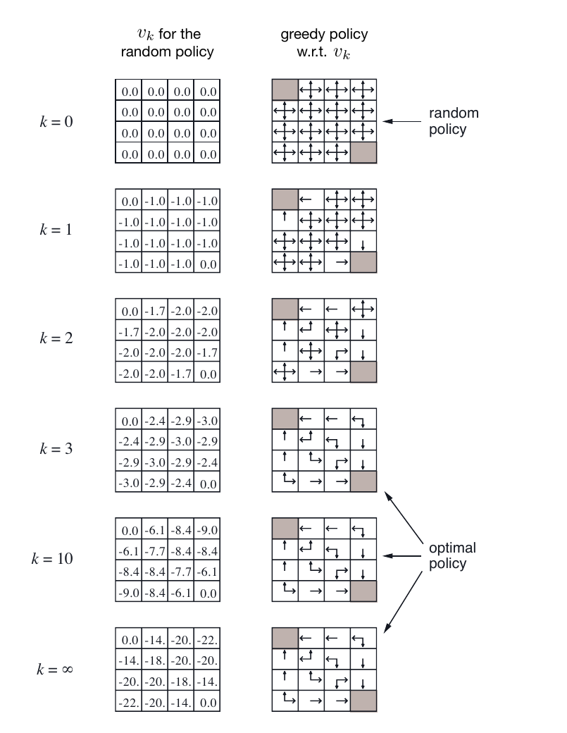
Source: Sutton and Barto, Reinforcement Learning: An Introduction, 2nd ed., Figure 4.1. The original book uses the CC BY-NC-ND 2.0 license.

For now, it is enough to look only at the left column. At $k=0$, except for terminal states, many cell values start from 0. After several iterations, positions near the terminal states change first, and farther positions are gradually pulled along. The numbers are not “the reward obtained immediately upon entering this cell.” They are “the expected total return from this cell onward under the current policy.”

Consider a minimal example: a three-cell corridor.

Environment rule table: records what happens in one step

Current state	Action	Next state	Reward
$S$	Move right	$M$	$-1$
$M$	Move right	$G$	$-1$
$G$	End	None	$0$

Value table: records how much it is probably worth from here onward

State $s$	Current estimate $V(s)$	Meaning
$S$	$-2$	Starting from $S$, two steps are expected
$M$	$-1$	Starting from $M$, one step is expected
$G$	$0$	Already at the terminal state; no future reward

The first table comes from the environment and tells us “what happens after one step.” In this corridor example, transitions are deterministic, so each row contains only one next state. If the same action may lead to multiple next states, the environment rule table must be written with probabilities, which is exactly $P(s'\mid s,a)$. The second table comes from the algorithm and stores the current estimate of long-term return. Reward is one-step; value is long-term. Reward is given by the environment; value must be estimated by the algorithm.

Notice that the $-2,-1,0$ in the second table are the results after computation is already correct. At the beginning, the algorithm usually does not know these answers. It may initialize the entire table to 0:

State $s$	Current estimate $V(s)$
$S$	$0$
$M$	$0$
$G$	$0$

The 0 here does not mean these states are truly worth only 0 points. It means “we do not know yet, so use 0 as the initial guess.” What later DP, MC, and TD methods do is continuously modify the right-hand column so that it gradually approaches the true $V^\pi$.

To summarize: the value table solves a very concrete problem: it gives the abstract value function a carrier that can be repeatedly updated. When the number of states is finite and enumerable, the value table is the most direct representation. When the state space is huge or continuous, this table cannot fit everything, and later we need function approximation and neural networks to replace it.

The same idea naturally extends to action values. A state-value table stores one number for each state; an action-value table stores one number for every “state-action pair,” namely $Q(s,a)$. The Q table in Section 3.5 is essentially the value table here extended from “one cell per state” to “one cell per action under each state.” Classic TD learning can be viewed as using experience to correct state predictions^[2]; Q-learning updates action values in a tabular setting with finite states, finite actions, and repeated sampling^[3].

From Equation to Update Rule

The previous subsection explained the role of the value table: every state has a location in the table, but the number inside is initially only a temporary estimate. The next real problem is: how should these numbers gradually become estimates closer to the true values?

Look at the Bellman equation from another angle. Earlier, when we wrote it, it looked like an “equality that the correct answer must satisfy”:

$$V^\pi(s)= \sum_a\pi(a\mid s) \left[ R(s,a)+\gamma\sum_{s'}P(s'\mid s,a)V^\pi(s') \right].$$

Both sides here use the true $V^\pi$, so the equation describes the relationship of the final answer. But at the beginning, the algorithm does not have the true $V^\pi$. It only has a temporary value table $V_k$. Therefore, the natural idea is: treat the right-hand side of the equation as a new target value, and use it to rewrite the old table.

Before answering how to rewrite it, distinguish two situations:

• The environment model is known: here “environment model” means the mathematical version of the environment rules: after taking action $a$ in state $s$, with what probability will we arrive at each next state $s'$, and how much reward will we obtain on average? In other words, we know the transition probability $P(s'\mid s,a)$ and reward $R(s,a)$, so we can directly use the Bellman equation to construct an update rule.
• The environment is a black box: we do not know this information. We can only actually take one step, observe one reward and one next state.

First look at the first situation.

For a fixed policy $\pi$, denote the old table as $V_k$. Now we no longer pretend that we already know the true $V^\pi$. Instead, we use $V_k(s')$ in the old table to estimate the value of next states:

$$\text{BellmanTarget}_k(s)= \sum_a\pi(a\mid s) \left[ R(s,a)+\gamma\sum_{s'}P(s'\mid s,a)V_k(s') \right].$$

This step means:

• The inner $\sum_{s'}P(s'\mid s,a)V_k(s')$ computes “the expected value of the next state after taking action $a$.”
• The outer $\sum_a\pi(a\mid s)$ averages over actions according to the current policy $\pi$.
• After adding $R(s,a)$ and discount factor $\gamma$, the result is “how much the old table thinks state $s$ should now be worth.”

The update rule is then direct:

$$V_{k+1}(s)\leftarrow \text{BellmanTarget}_k(s).$$

Doing this computation for all states produces a new round of the value table, $V_{k+1}$. This step is often called a Bellman backup: use the old estimate of the next state to update the current state in reverse.

Sometimes we do not directly replace the old value, but only move a small step toward the target:

$$V(s)\leftarrow V(s)+\alpha\left[\text{BellmanTarget}_k(s)-V(s)\right].$$

Here $\alpha$ is the learning rate. $\alpha=1$ means fully adopting the new target; $\alpha=0.1$ means moving the old value only 10% of the way toward the target. Whether we replace directly or move by a small step, the core idea is the same: the right-hand side of the Bellman equation gives the target, and the value table stores the current estimate.

Use a minimal example to verify this. To avoid being distracted by multiple states, shrink the value table to the minimum: the entire table has only one row, and the only state is $s$.

State $s$	Current estimate $V(s)$
$s$	$0$

Imagine there is only one slot machine A in front of you. Each round, you press the button, receive one reward, and then return to the same state $s$. The policy is fixed: always choose A. Now ask only one question:

Starting from this state and continuing forever, what is the discounted average total return?

The setting is:

• There is only one state, and after playing one round, we return to the same state.
• Always choose machine A.
• Machine A gives reward $+1$ with probability 60% and reward $-1$ with probability 40%.
• The discount factor is $\gamma=0.9$.

The one-step expected reward is:

$$R=0.6\times(+1)+0.4\times(-1)=0.2$$

Because after each round we are still in the same state, the next-state value still looks up the same cell in the value table, namely $V(s)$. According to the Bellman expectation equation:

$$V(s)=0.2+0.9V(s)$$

Analytic solution: solve the equation directly. $V(s)-0.9V(s)=0.2$, so $V(s)=2.0$. This $2.0$ is not a one-step reward. It is the number that the cell for state $s$ in the value table should ultimately approach, meaning “from now on, if we keep playing, the discounted average total return.”

Iterative method: if we do not want to, or cannot, solve the equation directly, we can also start from the initial value table $V_0(s)=0$ and perform one Bellman update each round, changing the cell for state $s$ into a new estimate:

$$V_{k+1}(s)\leftarrow R+\gamma V_k(s)$$

Compute the first few rounds by hand:

Round	Update formula	New value of $V(s)$ in the table
Initial	-	$0$
Round 1	$0.2+0.9\times0$	$0.2$
Round 2	$0.2+0.9\times0.2$	$0.38$
Round 3	$0.2+0.9\times0.38$	$0.542$
Round 4	$0.2+0.9\times0.542$	$0.6878$
Round 5	$0.2+0.9\times0.6878$	$0.81902$

Each round uses “immediate expected reward $0.2$ + discounted old value estimate” to obtain a new estimate. Because there is only one state, it looks like we are only updating one number. With multiple states, the same operation updates the whole value table cell by cell. At the beginning it is far from $2.0$, but it approaches gradually.

R = 0.2
gamma = 0.9
V = 0.0

for i in range(50):
    V = R + gamma * V

print(round(V, 6))

运行结果

1.998698

This is the basic shape of Bellman iteration: instead of computing the answer all at once, repeatedly apply the Bellman relationship so that the estimate gradually approaches the true value. Under a fixed policy $\pi$, this corresponds to iterative policy evaluation. If later we replace “averaging according to the policy” with “taking the maximum over actions,” it leads to value iteration in optimal control.

When the Environment Is a Black Box: TD Error

Return to the slot-machine example. There we could write $V(s)=0.2+0.9V(s)$ because two things were already known: the average reward each time is $0.2$, and after pressing the button we definitely return to the same state. In other words, we knew the environment rules, so we could directly compute “what happens next on average.”

Real tasks are usually not this convenient. The agent does not know where each action will lead, nor the probabilities of different outcomes. It can only actually take a step, see a reward, and see which state it lands in. TD error is used in this situation. First understand it as a reconciliation tool: compare “the target given by this one actual experience” with “the old estimate in the value table,” and see how much they differ.

If you do not fully understand this on the first reading, that is fine. The next section compares DP, MC, and TD side by side, and later algorithm chapters will repeatedly return to this concept. For now, grasp one distinction: when the model is known, we compute the average case; TD sees only the one case that just happened.

First look at the known-model form. Suppose we know the complete environment rules. Then we can write the exact Bellman target:

$$\sum_a\pi(a\mid s) \left[ R(s,a)+\gamma\sum_{s'}P(s'\mid s,a)V(s') \right].$$

Here $R(s,a)$ is not one realized reward, but an average reward; $P(s'\mid s,a)$ is not one realized next state, but the probability of each possible next state. The expression means: include all possible actions and all possible next states, then average according to their probabilities.

TD cannot do this. It does not have that probability table. It only knows what truly happened in the most recent step: the reward observed this time was $r$, and the next state reached this time was $s'$. Therefore, it first constructs a temporary target from this one experience:

$$\text{Target} = r + \gamma V(s')$$

The lowercase $r$ and $s'$ remind us that they are not the average laws of the environment, but one result just observed. This target may be too high or too low, but after many samples, these high and low deviations gradually cancel out.

The comparison is:

Method	Reward used	Next state used	Nature of target
Exact Bellman update	Expected reward $R(s,a)$	All possible $s'$, weighted by $P(s'\mid s,a)$	Exact expectation
TD update	This actual reward $r$	This actual next state $s'$	Noisy one-sample estimate

A numerical example makes it clearer. Suppose that after acting according to the current policy in state $s$, the environment has two possible outcomes:

Next state	Probability	This-step reward	Current value estimate
$s_1$	70%	$+1$	$V(s_1)=5$
$s_2$	30%	$-1$	$V(s_2)=0$

Let $\gamma=0.9$. If the model is known, we include both possibilities:

$$\text{BellmanTarget} =0.7\times(1+0.9\times5)+0.3\times(-1+0.9\times0) =3.55.$$

This is the exact Bellman update. It is like holding an environment manual: we know what outcomes may happen from $s$ and the probability of each, so we can compute the average target $3.55$ at once.

TD is in a different position. It does not have this manual, and it is not actively sampling outcomes with 70% and 30% by itself. “Sampling” only means that the agent actually took one step and the environment gave it one result. If the environment naturally has the pattern “most of the time go to $s_1$, sometimes go to $s_2$,” then when repeatedly starting from $s$, the agent will naturally see $s_1$ more often and $s_2$ occasionally. But in each update, TD uses only the single experience in front of it.

Suppose the value table currently has $V(s)=3$, and the learning rate is $\alpha=0.1$.

If this time it really reached $s_1$ and received reward $r=1$, TD computes:

$$\text{TD Target}=1+0.9\times5=5.5,$$

$$\delta=5.5-3=2.5,$$

Then it adjusts $V(s)$ upward a little:

$$V(s)\leftarrow 3+0.1\times2.5=3.25.$$

If another time it really reached $s_2$ and received reward $r=-1$, TD computes:

$$\text{TD Target}=-1+0.9\times0=-1,$$

$$\delta=-1-3=-4,$$

Then it adjusts $V(s)$ downward a little:

$$V(s)\leftarrow 3+0.1\times(-4)=2.6.$$

Put the two cases together:

What really happened this time	TD Target	TD error $\delta$	Updated $V(s)$
Reached $s_1$, reward $+1$	$5.5$	$2.5$	$3.25$
Reached $s_2$, reward $-1$	$-1$	$-4$	$2.6$

There is an important detail here: TD does not guarantee that every single update moves closer to the average target.

In this example, the exact Bellman target is $3.55$, while the current $V(s)=3$, so the difference is $0.55$. If this time we reached $s_1$, the updated value becomes $3.25$, which is indeed closer to $3.55$. But if this time we reached $s_2$, the updated value becomes $2.6$, which is farther from $3.55$.

This is not a contradiction. It is normal TD behavior. TD corrects the value table using only the experience in front of it, so one “bad outcome” pulls the estimate down, and one “good outcome” pushes it up. A single update may move in the wrong direction; what matters is the average direction over many updates.

Combine the two updates according to the environment’s own probabilities:

$$0.7\times3.25+0.3\times2.6=3.055.$$

That is, if we start from $V(s)=3$, the “average position” after the next TD update is $3.055$. It still does not jump directly to $3.55$, but it is already closer to $3.55$ than $3$ was.

Similarly, from the TD error perspective:

$$0.7\times2.5+0.3\times(-4)=0.55.$$

The average TD error is positive, which means that over the long run, the current $V(s)=3$ is too low and should be adjusted upward. It is just that each actual experience does not necessarily move in that direction.

The point of this table is not that “the agent should sample according to 70% and 30%.” It is that TD only looks at one real experience each time. Common outcomes participate in updates more frequently, and rare outcomes participate less frequently. After many updates accumulate, the average direction gradually approaches the probability-weighted Bellman target above.

This $\delta$ is the Temporal Difference Error, usually called the TD Error. It measures how far the “one-step target” is from the “current estimate”:

$$\delta = \underbrace{r + \gamma V(s')}_{\text{Bellman target}} - \underbrace{V(s)}_{\text{current estimate}}$$

Why is it called “temporal difference”? Because it compares prediction differences between two neighboring states in a time sequence: when standing at $s$, we have an old prediction; after moving to $s'$, the term $r+\gamma V(s')$ gives a new target.

Its meaning is direct:

TD Error	Meaning	How to adjust
$\delta>0$	The target is higher than the current estimate, so we underestimated	Increase $V(s)$
$\delta<0$	The target is lower than the current estimate, so we overestimated	Decrease $V(s)$
$\delta=0$	Under this sample, the target and estimate agree	Almost no adjustment needed

The simplest update formula is:

$$V(s)\leftarrow V(s)+\alpha\delta.$$

The $3.25$ and $2.6$ in the two branches above are exactly the results of this formula when $\alpha=0.1$.

This is the basic move of TD learning: every time the agent takes a step, it uses “the one step actually experienced + the next-state estimate” to correct the current-state estimate. After many samples, the noise of single samples is averaged out, and the value table gradually approaches the true $V^\pi$.

DP, MC, and TD handle different environment conditions and information assumptions. The next section, Classic Methods at a Glance: DP, MC, and TD, compares them specifically.

Section Summary

This page has many formulas, but only one main thread:

1. $V^\pi(s)$ is the average long-term return obtained by starting from state $s$ and acting according to policy $\pi$.
2. Return can recurse: $G_t=r_t+\gamma G_{t+1}$.
3. Therefore value can also recurse: current value equals immediate reward plus next-state value.
4. If the policy is fixed, we obtain the Bellman expectation equation.
5. If the best action is chosen at every step, we obtain the Bellman optimality equation.
6. In finite-state problems, $V(s)$ can be stored as a value table, giving every state an updatable number.
7. If we only have sampled data, we use the Bellman target and TD Error to gradually correct $V(s)$ in the value table.

$V(s)$ can already tell you “whether this situation is good,” but there are still two gaps at this point.

The first gap is: if we do not know the environment model, how do we estimate $V$? The Bellman expectation equation contains $P(s'\mid s,a)$ and $R(s,a)$, but in real tasks we often only obtain sampled trajectories one by one. The next section discusses DP, MC, and TD, which are three ways to estimate value from models or data.

The second gap is: $V$ does not directly tell you which action to choose. If $V(s)=80$, you only know the current situation is good, but you do not know whether to go left, go right, or stay still. A more direct approach is to score each action as well:

$$Q(s,a)$$

There is no need to expand $Q$ yet. For now, just remember the division of labor between the two tables: the value table $V(s)$ scores states, while the action-value table $Q(s,a)$ scores “first taking action $a$ in state $s$.” If the environment model is known, meaning we know how each action affects the next state and reward, we can use the $V$ table for one-step lookahead to compare actions. If the environment model is unknown, directly learning the $Q$ table is often more convenient, because it stores the long-term consequences of each action directly.

So the next sequence is: first read DP, MC, and TD to solve “how to estimate $V$”; then enter Action-Value Function to solve “how to use value to choose actions.”

References

---

1. Sutton, R. S., & Barto, A. G. (2018). Reinforcement Learning: An Introduction (2nd ed.). MIT Press. Part I of the book is titled “Tabular Solution Methods,” and Chapter 4, Figure 4.1 shows the policy-evaluation process of writing state values directly in Gridworld cells. MIT Press Open Access page: https://mitpress.mit.edu/9780262039246/reinforcement-learning/; author-hosted PDF: http://incompleteideas.net/book/RLbook2020.pdf. ↩︎

2. Sutton, R. S. (1988). Learning to predict by the methods of temporal differences. Machine Learning, 3(1), 9-44. DOI: https://doi.org/10.1007/BF00115009. ↩︎

3. Watkins, C. J. C. H., & Dayan, P. (1992). Q-learning. Machine Learning, 8, 279-292. DOI: https://doi.org/10.1007/BF00992698; author page: https://www.gatsby.ucl.ac.uk/~dayan/papers/wd92.html. ↩︎