6.4 Hands-on: Pendulum Swing-Up and Balance

Goal of this section: Train Pendulum-v1 with A2C, understand why continuous-action Actor-Critic outputs a Gaussian distribution, and see how the Critic helps the Actor learn stable control in continuous spaces.

Code for this section: actor_critic_pendulum.py · render_pendulum.py · requirements.txt

Earlier in the chapter, we used CartPole and LunarLander to understand RL where the agent picks one of a few discrete actions. Those action spaces fit DQN naturally and are easy to explain via a Softmax policy: left, right, fire, or do nothing, each action with a clear probability.

Pendulum-v1 changes the problem. The agent is not choosing among buttons. It must apply a continuous torque to a rod. That torque could be -2, or 0.17, or 1.843. The action is no longer a few discrete bins; it is the entire real interval $[-2, 2]$. This is the new problem that Actor-Critic was designed to solve: when there are infinitely many action candidates, how should a policy express "this is what I want to do"?

6.4.1 Task Intuition: Not Picking a Button, but Controlling Torque

The Pendulum setup is simple. A rod hangs from a pivot. At each step the agent applies a torque, and the goal is to swing the rod up to the upright position and keep it there.

The environment provides a 3-dimensional state:

State component	Meaning
$\cos\theta$	cosine of the rod angle
$\sin\theta$	sine of the rod angle
$\dot\theta$	angular velocity of the rod

The action is a 1-dimensional continuous value:

Action component	Meaning
$a$	torque applied to the pivot, in the range $[-2, 2]$

The reward function can be understood as the sum of three penalties:

$$r = -(\theta^2 + 0.1\dot\theta^2 + 0.001a^2)$$

Here $\theta$ is the angle away from upright, $\dot\theta$ is the angular velocity, and $a$ is the torque action. In plain terms: the further the rod deviates from upright, the more penalty; the faster it spins, the more penalty; even using a large torque carries a small penalty. The ideal case — rod upright, near-zero velocity, small torque — yields a per-step reward close to 0.

Because of this formulation, the cumulative return on Pendulum is typically negative. A random policy often scores around -1200 to -900. A well-trained policy can push toward -500, -300, or even closer to 0. When reading these curves, don't ask "why isn't the reward positive?"; instead, watch whether it climbs from deeply negative values toward 0.

6.4.2 Why DQN Does Not Fit This Task

Let's start from what we already know: DQN. DQN learns $Q(s,a)$ and acts by

$$a^* = \arg\max_a Q(s,a)$$

This formula is natural for discrete action spaces. CartPole has two actions; we compute $Q(s,\text{left})$ and $Q(s,\text{right})$ and pick the larger one.

But Pendulum's action is any real number in $[-2, 2]$. Strictly computing $\arg\max_a Q(s,a)$ means comparing $Q$ values across infinitely many torque values. This is not a "let's just try a few more actions" problem — the very representation of the action has changed.

One naive fix is to discretize $[-2, 2]$ into, say, 21 bins:

$$\{-2.0,-1.8,-1.6,\ldots,1.8,2.0\}$$

This lets DQN barely run, but it creates two problems. First, control precision is limited by the bin width: the agent can never output a torque like 0.37. Second, the number of bins explodes as soon as the action dimension grows. Pendulum has only 1 action dimension, so 21 bins is manageable. But BipedalWalker has 4 continuous action dimensions; with 21 bins each, the total action count becomes $21^4 = 194{,}481$.

The real issue, then, is not "can DQN get a few more output heads?" It is this: continuous control requires a policy that can directly generate continuous actions.

6.4.3 Continuous Actor: Output a Gaussian Distribution

A discrete policy outputs a probability for each action:

$$\pi(a|s) = [0.2, 0.8]$$

A continuous policy cannot enumerate all actions because there are infinitely many. The natural alternative is to have the Actor output the parameters of a probability distribution. For Pendulum, the most common choice is a Gaussian:

$$a \sim \mathcal{N}(\mu_\theta(s), \sigma_\theta(s)^2)$$

Here $\mu_\theta(s)$ is the mean that the policy network outputs given state $s$, and $\sigma_\theta(s)$ is the standard deviation for action sampling. In plain terms: the Actor does not say "the action shall be exactly 0.7". It says "I tend to apply torque around 0.7, while keeping some randomness for exploration."

The network in code looks like this:

class ActorCriticContinuous(nn.Module):
    def __init__(self, state_dim=3, action_dim=1, hidden_dim=128):
        super().__init__()
        self.shared = nn.Sequential(
            nn.Linear(state_dim, hidden_dim),
            nn.ReLU(),
            nn.Linear(hidden_dim, hidden_dim),
            nn.ReLU(),
        )
        self.mu_head = nn.Linear(hidden_dim, action_dim)
        self.log_std = nn.Parameter(torch.zeros(action_dim))
        self.value_head = nn.Linear(hidden_dim, 1)

    def forward(self, state):
        features = self.shared(state)
        mu = torch.tanh(self.mu_head(features)) * 2.0
        std = torch.exp(self.log_std).expand_as(mu)
        value = self.value_head(features)
        return mu, std, value

Three design choices are worth noting.

First, mu_head outputs the action mean. Since Pendulum's legal action range is $[-2, 2]$, the code uses tanh to squash the output into $[-1, 1]$, then multiplies by 2.

Second, log_std is a learnable parameter. Instead of learning $\sigma$ directly, we learn $\log\sigma$ and recover a positive standard deviation via exp. This avoids the standard deviation ever becoming negative.

Third, value_head is the Critic, outputting $V(s)$. The shared feature trunk feeds both the Actor head and the Critic head. This is exactly the Actor-Critic architecture described throughout the chapter: the Actor decides how to act, the Critic judges roughly how good the current situation is.

6.4.4 How the Critic Provides a Learning Signal for the Actor

An Actor alone is not enough. We need to know whether a given action was "better or worse than expected." The Critic provides this reference.

At each step, the Critic estimates the current state value $V(s_t)$. Meanwhile, the next reward and the next state value form a TD target:

$$y_t = r_t + \gamma V(s_{t+1})$$

The TD error measures the gap between the actual outcome and the original estimate:

$$\delta_t = y_t - V(s_t)$$

This $\delta_t$ is the advantage estimate used in the Actor update. If $\delta_t > 0$, the action produced a better result than the Critic expected — the Actor should increase its probability. If $\delta_t < 0$, the result was worse than expected — the Actor should lower its probability.

In code, the core update is:

td_target = reward + gamma * not_done * next_value
advantage = td_target - value

actor_loss = -(log_prob * advantage.detach())
critic_loss = advantage.pow(2).mean()
loss = actor_loss + 0.5 * critic_loss - 0.001 * entropy

The actor_loss has a negative sign because the optimizer performs gradient descent by default. We want: when advantage is positive, increase log_prob; when advantage is negative, decrease log_prob. Turned into a loss, this becomes minimizing -(log_prob * advantage).

The critic_loss pushes the Critic's estimate toward the TD target. The final entropy term encourages the policy to retain some exploration and prevents the standard deviation from collapsing too early.

6.4.5 Running the Training

Install dependencies:

pip install -r code/chapter06_actor_critic/requirements.txt

A quick smoke test to confirm the script runs:

python code/chapter06_actor_critic/actor_critic_pendulum.py \
  --total-timesteps 20000

This section's script uses Stable-Baselines3's A2C (Advantage Actor-Critic) implementation. A2C is still Actor-Critic: the Actor learns a continuous-action policy, the Critic learns $V(s)$. The engineering additions — parallel environments and return normalization — simply make this teaching experiment easier to reproduce. Run the full training:

python code/chapter06_actor_critic/actor_critic_pendulum.py \
  --total-timesteps 300000

The training script generates a model, normalization statistics, and three curves under output/:

File	Meaning
actor_critic_pendulum.zip	trained A2C model
actor_critic_pendulum_vecnormalize.pkl	observation and reward normalization
actor_critic_pendulum_reward.png	episode reward curve
actor_critic_pendulum_entropy.png	policy entropy loss curve
actor_critic_pendulum_loss.png	Actor/Critic loss curves

To copy the plots into the course site:

cp output/actor_critic_pendulum_*.png docs/chapter06_actor_critic/images/

After training, you can render a replay GIF:

python code/chapter06_actor_critic/render_pendulum.py \
  --model output/actor_critic_pendulum.zip \
  --output output/pendulum_actor_critic.gif

6.4.6 Experimental Results: First Learn to Swing Up, Then Learn to Stabilize

Here are the results from a 300k-step training run. Since A2C is still an on-policy Actor-Critic — each batch of data is used once and discarded — the per-episode variance is higher than what you will see with PPO in Chapter 7. Focus on the moving-average trend, not any single episode's spike or dip.

Figure 6.4-1: Pendulum replay after A2C training. This episode scored roughly -761; it reaches near-upright but is not yet near-optimal stable control.

Figure 6.4-2: Episode reward curve. Light blue shows raw returns, dark blue is a 20-episode moving average, and the green dashed line marks the A2C baseline of -800.

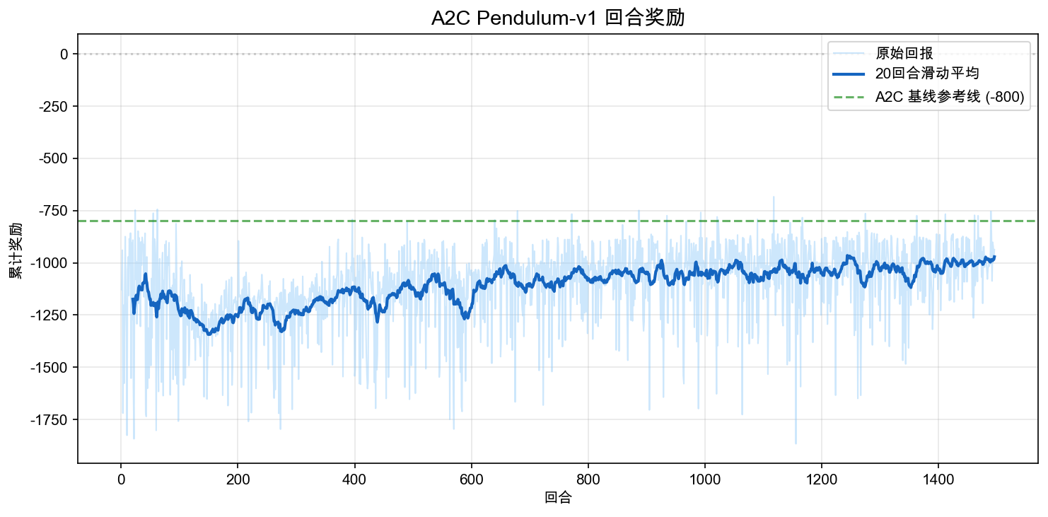
The deterministic evaluation for this run is approximately -780 ± 39 (over 20 episodes), with the best single episode around -750. It is more stable than a random or early policy, but it is not yet near-optimal pendulum control. That is intentional: the goal of this section is not to push Pendulum to the best possible score, but to use a small enough continuous-control task to clearly walk through the "Gaussian Actor + value Critic + advantage update" pipeline.

The curve reveals three phases:

• Early training: rewards often hover around -1200. The rod mostly swings near the bottom with no structured action pattern.
• Mid training: the moving average rises slowly. The policy begins to discover effective torque patterns, but cannot yet reliably keep the rod upright.
• Late training: rewards settle roughly in the -1000 to -800 range. The policy is clearly better than its starting point, but control near the upright position remains unsteady.

Pendulum learning is not like CartPole, where perfect scores appear quickly. Here the action requires both direction and magnitude. Too little torque, and the rod never swings up. Too much torque, and it overshoots the top. This is exactly the difficulty of continuous control: the policy is not choosing "left or right" — it is choosing a precise force magnitude at every step.

6.4.7 Policy Entropy: How Exploration Gradually Narrows

One advantage of a Gaussian policy is that we can directly observe exploration intensity. A larger standard deviation $\sigma$ means more dispersed action sampling; higher policy entropy means a more random action distribution.

Figure 6.4-3: Policy entropy loss. SB3 records entropy_loss, i.e., negative entropy. As the curve climbs toward 0, the true entropy is declining.

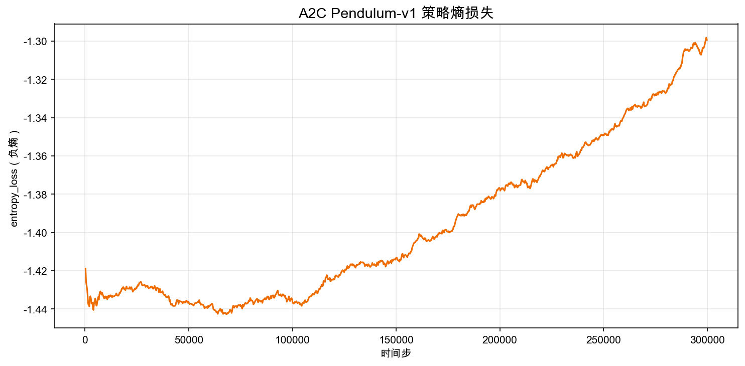
Looking at the learning process, the policy initially needs substantial randomness. It does not yet know which direction to push, nor how to decelerate when approaching the upright position. As the Critic's advantage signals become more reliable, the Actor gradually concentrates probability mass around effective actions, and the true policy entropy slowly drops.

But entropy should not drop too fast. If the action distribution becomes too narrow early on, the policy may prematurely lock into an ineffective pattern — for example, only producing tiny twitches that never swing the rod up. This is why algorithms like A2C and PPO usually monitor policy entropy.

In this section's configuration, ent_coef=0.0. This does not mean entropy is unimportant; it means Pendulum's Gaussian policy already has inherent sampling noise. For more difficult continuous-control tasks, adding an explicit entropy bonus is usually more reliable.

6.4.8 Loss Curves: What the Actor and Critic Are Each Doing

The reward curve tells us whether performance is improving; the loss curves help us understand whether training is stable.

Figure 6.4-4: Actor/Critic loss curves. Online Actor-Critic losses are typically noisier than supervised learning losses. Focus on whether they diverge over the long run.

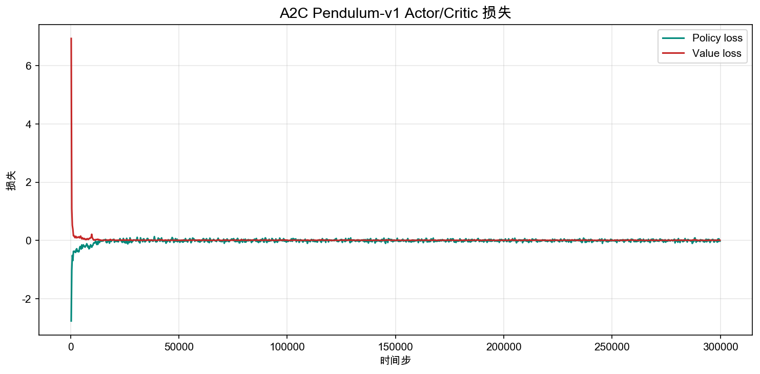
The Critic loss comes from the squared TD error:

$$(\delta_t)^2 = (r_t + \gamma V(s_{t+1}) - V(s_t))^2$$

If the Critic loss stays large over an extended period, it means the value estimates are unstable, and the advantage signals reaching the Actor will also be unreliable. The Actor loss is related to log_prob * advantage; its value does not necessarily decrease monotonically because the policy changes at every step and the sampling distribution shifts along with it.

This is why RL cannot be monitored by loss alone, unlike an ordinary classification task. A more reliable evaluation order is: first check whether episode reward is rising, then check whether the Critic loss diverges over the long run, and finally check whether entropy and standard deviation collapse prematurely.

6.4.9 Common Failures and Hyperparameter Tuning

If Pendulum fails to learn, go through these checks in order.

First, confirm the training budget is sufficient. --total-timesteps 20000 only verifies that the code path runs; it does not demonstrate algorithmic performance. Start full training from at least 300k steps.

Second, confirm that VecNormalize is enabled. Pendulum's raw reward scale is fairly large, and the Critic has a harder time fitting raw returns directly. The script saves actor_critic_pendulum_vecnormalize.pkl; make sure to load it during evaluation and rendering as well.

Third, watch whether the Critic loss explodes persistently. If the TD error stays large for a long time, the advantage signals reaching the Actor will be extremely noisy. Try lowering the learning rate or increasing the number of parallel environments to improve sample stability.

Fourth, check whether the actions are frequently stuck at the boundaries. If the action is consistently -2 or 2, the policy has learned "push hard" but not how to decelerate near the upright position. Continue training, or use a more stable policy optimization method like PPO in the next chapter.

Common hyperparameter reference:

Parameter	This section's setting	What happens if it is off
learning_rate	7e-4	too high causes oscillation; too low learns too slowly
n_steps	32	too short gives noisy advantages; too long reduces update frequency
gamma	0.99	too low focuses on near-term swing, ignoring staying upright
num_envs	8	too few collects samples slowly; too many adds overhead
VecNormalize	enabled	without it the Critic has a harder time fitting raw returns

6.4.10 Section Summary

Pendulum takes us from discrete actions to continuous actions. The real change is not that the environment is more complex; it is that the policy representation changes: the Actor no longer outputs Softmax probabilities over a few actions. Instead, it outputs the mean and standard deviation of a Gaussian distribution, and a continuous torque is sampled from that distribution.

The Critic provides a baseline in this process. It estimates the value of the current state with $V(s)$, then uses the TD error to tell the Actor: was that last action better or worse than expected? This way, the policy can gradually shift probability mass toward more effective control signals within the continuous action space.

At the same time, this experiment exposes the limitations of vanilla Actor-Critic: it explains the basic mechanics of continuous control, but its sample efficiency and stability are not ideal. The next chapter's PPO adds a mechanism — capping how much the policy can change per update — on top of the same Actor-Critic framework. That mechanism is exactly what makes complex continuous-control tasks reliably trainable.

In the next section, we take the same ideas to a more complex robot task: Hands-on: BipedalWalker Locomotion.