2.2 Training Metrics

In Section 2.1, we derived the DPO loss. Now let's come back to the experiment and interpret the metrics that DPOTrainer.train() prints during training.

Compared to classic RL benchmarks like CartPole, preference alignment does not have an environment-provided scalar reward per step. As a result, the training log exposes a richer set of internal signals.

When you run trainer.train(), you will typically see logs like:

Step  Training Loss  Rewards/Margins  Rewards/Chosen  Rewards/Rejected  Rewards/Accuracies
  5       0.6821          0.0312          -0.0156          -0.0468              0.52
 10       0.6543          0.1247           0.0891          -0.0356              0.58
 15       0.5987          0.3421           0.2314          -0.1107              0.72
 ...
 45       0.2103          1.5632           0.9201          -0.6431              0.92

If you also log to SwanLab or TensorBoard, you can inspect the same signals as curves. We'll go through each column and explain what it means and how to diagnose problems.

Training Loss

Training Loss is the DPO loss $\mathcal{L}_{\text{DPO}}$ evaluated on the current minibatch.

At the start of training, the policy $\pi_\theta$ is usually initialized from the same checkpoint as the reference model $\pi_{\text{ref}}$. That means the ratio terms are close to 1, the log ratios are close to 0, and the margin inside the sigmoid is near 0.

Since $\sigma(0) = 0.5$, the initial loss is roughly:

$$-\ln(0.5) = \ln 2 \approx 0.693$$

This explains why early logs are often near $0.69$. A steadily decreasing loss that later stabilizes is usually a healthy sign.

But "lower is always better" is not the right mindset here. If the loss collapses too quickly toward 0, it can indicate overfitting: the model memorizes preference pairs instead of learning a robust preference notion.

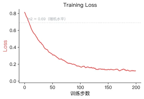
Typical healthy behavior:

• starts near $\ln 2 \approx 0.69$
• decreases over time
• stabilizes at some positive value (label noise prevents it from reaching 0)

Common failure patterns:

Symptom	Likely Cause	Severity
Loss stays near 0.69	learning rate too low, data issues	high
Loss drops then spikes	learning rate too high, batch quality instability	medium
Loss quickly goes to ~0	overfitting to preference data	medium

If the preference labels are wrong, what happens to the loss?

The loss can still decrease "normally". The policy is simply fitting the preference relations you provided; it does not know which side is ethically or factually correct. If the data says that toxic responses are chosen, the model will learn that.

This is the central rule of post-training: data quality dominates. Garbage in, garbage out.

Reward Margin

Rewards/Margins corresponds to the margin term inside the sigmoid. It directly measures how strongly the policy prefers the chosen answer over the rejected one:

$$\text{Margin} = \beta \ln \frac{\pi_\theta(y_w \mid x)}{\pi_{\text{ref}}(y_w \mid x)} - \beta \ln \frac{\pi_\theta(y_l \mid x)}{\pi_{\text{ref}}(y_l \mid x)}$$

A healthy margin curve usually starts near 0 and gradually increases, then stabilizes.

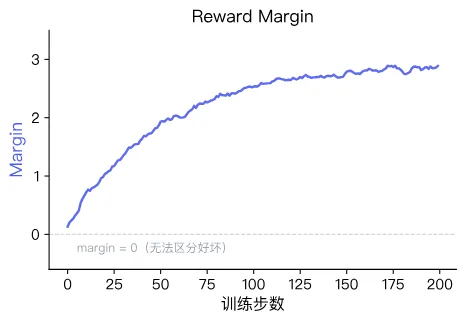
Interpretation guide:

• margin positive and increasing: the model is separating chosen vs rejected more confidently
• margin negative or oscillating near 0: the model is struggling to learn the preference relation

Common causes of poor margins include: ambiguous preference pairs, extreme length imbalance between chosen and rejected, and unstable hyperparameters.

What happens if we change beta from 0.1 to 1.0?

beta is the regularization strength controlling how far the policy is allowed to drift from the reference model. In 3-train_dpo.py, it is set by DPOConfig(beta=0.1).

• if beta is large (e.g. 1.0): the policy is heavily constrained, so margins may grow slowly or barely grow
• if beta is tiny (e.g. 0.01): the policy may drift too far, sometimes learning degenerate hacks that optimize the objective but hurt response quality

Suggested exercise: run the same training with beta = 0.01 and beta = 0.5, and compare the margin curves.

Reward Accuracy

Rewards/Accuracies measures how often the policy assigns higher implicit reward to the chosen response than to the rejected response (on the current batch). In other words, it is a ranking accuracy:

• near 0.5: close to random guessing
• rising toward 0.8 to 0.95: the model is learning the preference relation

Accuracy is a coarse, binary signal ("chosen wins or not"). Margin is a finer, continuous signal ("by how much"). In a healthy run, they tend to improve together: accuracy rises and margin grows.

If accuracy is high but margin stays tiny, it can indicate the model can barely rank correctly, but with low confidence separation.

Chosen Reward vs Rejected Reward

Margin is a difference. Looking at only the difference can hide important dynamics.

The margin might increase because:

• chosen reward increases while rejected reward stays flat
• rejected reward decreases while chosen reward stays flat
• both change, but chosen changes more

These scenarios have very different meanings. That is why TRL logs both:

$$r_{\text{chosen}} = \beta \ln \frac{\pi_\theta(y_w \mid x)}{\pi_{\text{ref}}(y_w \mid x)}, \quad r_{\text{rejected}} = \beta \ln \frac{\pi_\theta(y_l \mid x)}{\pi_{\text{ref}}(y_l \mid x)}$$

A healthy trend is:

• $r_{\text{chosen}}$ gradually increases
• $r_{\text{rejected}}$ gradually decreases

If both increase or both decrease, you need to interpret them together with the loss and margin.

Extra: expanding the log ratio

For the chosen response:

$$\beta \ln \frac{\pi_\theta(y_w \mid x)}{\pi_{\text{ref}}(y_w \mid x)} = \beta \ln \pi_\theta(y_w \mid x) - \beta \ln \pi_{\text{ref}}(y_w \mid x)$$

Since $\pi_{\text{ref}}$ is fixed, changes in this term come entirely from $\ln \pi_\theta(y_w \mid x)$. TRL often logs logps/chosen and logps/rejected which are batch means of these log-probabilities; they can be useful for debugging.

---

Quick Reference Table

Metric	TRL log key	Healthy behavior	Red flags
Training Loss	loss	decreases from ~ln2 then stabilizes	stuck near 0.69; collapses to ~0
Reward Margin	rewards/margins	increases from ~0 then stabilizes	negative; oscillates near 0
Reward Accuracy	rewards/accuracies	rises from ~0.5 to ~0.8-0.95	stays near 0.5
Chosen Reward	rewards/chosen	increases	decreases or flat
Rejected Reward	rewards/rejected	decreases	increases

---

Chapter Summary

In Chapter 2, we accomplished:

1. Ran modern preference tuning: applied DPO to a 0.5B instruct model and reduced sycophancy within minutes of training.
2. Placed DPO inside the post-training pipeline: clarified the sequence Pre-training → SFT → Alignment, and where DPO fits.
3. Derived the DPO loss: saw how preference optimization can be expressed as a direct, sigmoid-based contrastive loss with a reference model.
4. Learned how to read metrics: understood Training Loss, Reward Margin, Reward Accuracy, and Chosen/Rejected rewards.

Whether it is CartPole in Chapter 1 or language alignment in this chapter, the central theme is the same: learn to make better decisions. Next, we move into the theory part and systematically build the mathematical foundations of reinforcement learning.

References