3.8 Reward Functions: Where Does the Optimization Objective Come From?

In the previous sections, we discussed value estimation methods and how data is collected. But whether we are doing DP, MC, or TD, and whether we are on-policy or off-policy, the target of every update ultimately comes from the same upstream source: the reward function.

The last section answered “where does the data come from.” In this section, we go one step further upstream and ask: how does the reward determine the direction of optimization, and why is it so hard to write a good reward?

Core Concept

The reward function defines “what is worth pursuing.” The algorithm does not see human intent; it only sees a scalar signal. If that signal is misaligned with the real objective, the stronger the optimization, the larger the deviation.

Let’s start with a tiny grid world to see how rewards change the task. The agent starts at the bottom-left and aims to reach the terminal goal at the top-right. Actions are up/down/left/right. We can write three different reward rules:

Reward Rule	Reward Per Step	Reaching Goal	Hitting Wall / Out of Bounds
Rule A	$0$	$+1$	$0$
Rule B	$-0.01$	$+1$	$0$
Rule C	$+0.02$	$+1$	$0$

These three environments have exactly the same map, states, and actions; the only thing that changes is the reward. Rule A cares only about whether the goal is eventually reached. Rule B additionally tells the agent that “taking fewer steps is better.” Rule C, however, accidentally tells the agent that “as long as you stay alive and keep moving, you get points.” Without a time limit, under Rule C the agent may learn to loop near the goal, because looping keeps collecting reward and can be “more profitable” than finishing quickly.

This highlights the most important fact about rewards: in the same environment, changing the reward changes the task as the agent perceives it. The state and action spaces describe what the agent can do. The transition probabilities describe what happens after it acts. The reward function describes what outcomes are worth pursuing.

The Role of the Reward Function

In the MDP 5-tuple $\langle \mathcal{S}, \mathcal{A}, P, R, \gamma \rangle$, rewards are commonly written as

$$R(s,a)$$

or, when rewards also depend on the next state, as

$$R(s,a,s').$$

The meaning is straightforward: when the agent chooses action $a$ in state $s$, the environment transitions to some next state $s'$, and this one-step transition produces an immediate scalar feedback signal (a real number).

What reinforcement learning truly maximizes is not a single-step reward, but the discounted return from the current time onward:

$$G_t=R_{t+1}+\gamma R_{t+2}+\gamma^2R_{t+3}+\cdots .$$

Here $\gamma$ is the discount factor. The closer $\gamma$ is to 1, the more the agent cares about the distant future; the smaller $\gamma$ is, the more it prefers immediate reward. In one sentence: the reward function scores each step, and the return aggregates those scores into a long-term objective.

This also explains why reward design determines behavior. The algorithm does not see the true human intention; it sees only this scalar signal. In our minds, we want “keep the pole upright stably,” “get to the maze exit,” or “give the user a helpful answer.” What the algorithm actually optimizes is the expected sum of numbers. If the numbers are not aligned with the intention, then the stronger the optimizer, the faster the misalignment can be amplified.

To understand reward, we also need to separate it from the value function from the previous section. In Section 3.3 we defined the state value function:

$$V^\pi(s)=\mathbb{E}_\pi[G_t\mid S_t=s].$$

Reward $R$ is the immediate signal provided by the environment after a one-step transition. Value $V^\pi$ is an estimate of how much long-term return can be obtained from a state under policy $\pi$. Reward is part of the task specification; value is a quantity computed by the learning algorithm from rewards and experience.

Return to the three-cell corridor from Section 3.3:

$$S\xrightarrow{-1}M\xrightarrow{-1}G.$$

The immediate reward from $S$ to $M$ is $-1$, and from $M$ to $G$ is also $-1$. If $\gamma=1$, then

$$V(S)=-2,\qquad V(M)=-1,\qquad V(G)=0.$$

These numbers are not rewards directly given by the environment. They are the long-term evaluation obtained by aggregating future rewards. If we changed each step reward from $-1$ to $+1$, the values would change completely, and the policy preference would change as well. A value function has no meaning independent of the reward definition; it is always “value under a particular reward.”

Signal Shapes

Once the role of reward in an MDP is clear, the next question is: what does the reward signal look like? Different signal shapes directly affect how hard learning is and what kinds of behaviors emerge.

The most conservative reward design looks only at the final outcome. For example, in a maze we can give $+1$ upon reaching the exit and $0$ otherwise:

$$R(s,a,s')= \begin{cases} +1, & s'\text{ is the goal state},\\ 0, & \text{otherwise}. \end{cases}$$

This is called a sparse reward. The advantage is that it is clean: we almost never hard-code our process preferences; we only tell the agent what the terminal objective is. The disadvantage is equally clear: the learning signal arrives too rarely. In a large maze, the agent may wander randomly for thousands of steps without ever reaching the exit, and the entire trajectory is all zeros. It knows it did not succeed, but it has no clue which steps were “closer to success.”

In contrast, a dense reward provides feedback at every step. For example, in a grid world we can reward the change in distance to the goal:

$$R_{\text{dense}}(s,a,s')=d(s,\text{goal})-d(s',\text{goal}).$$

Here $d(s,\text{goal})$ denotes the distance from state $s$ to the goal. If the next state is closer to the goal, the difference is positive; if it is farther, the difference is negative. The meaning is: do not wait until the terminal state to provide feedback; at each step, tell the agent whether it moved toward the goal.

Another common case is delayed rewards. Rewards are not completely sparse, but the key feedback arrives only after a long delay. In CartPole, each step receives $+1$ as long as the pole has not fallen, and the episode ends only at failure. Superficially, every step has a reward. But the real cause of failure may have occurred dozens of steps earlier: a slightly wrong push direction gradually destabilizes the system, and only later does the pole fall. Game tasks and LLM generation are similar. A preference score for an entire answer may be given only after the whole text finishes, yet the mistake that caused the low score may have appeared in the first sentence.

So “sparse,” “dense,” and “delayed” are not mutually exclusive labels. They describe the shape of the learning signal: how often it appears, how early it arrives, and whether it can clearly indicate which steps are good and which are bad.

Reward Shaping

Sparse rewards are clean but hard to learn from; dense rewards are easier to learn from but can introduce bias. Can we get the learning efficiency of dense signals without changing the original objective? Reward shaping aims to do exactly that.

The core idea is to add a shaping term $F(s, s')$ on top of the original reward $R$, so that the agent receives extra feedback at each step:

$$R'(s, a, s') = R(s, a, s') + F(s, s').$$

The question is how to design $F$. A poor shaping term can completely change the optimal policy. The earlier “positive per-step reward leads to looping” is a classic shaping side effect. Ng, Harada, and Russell (1999) proved that if the shaping term satisfies a potential-based form (Potential-Based Reward Shaping, PBRS), the optimal policy is invariant under the transformation^[1]:

$$F(s, s') = \gamma \Phi(s') - \Phi(s).$$

Here $\Phi(s)$ is a potential function defined on the state space. The interpretation is intuitive: moving from lower potential to higher potential yields positive feedback; moving the other way yields punishment. The key point is that this shaping form is equivalent to adding a state-dependent shift to the $Q$ function, without changing the relative ordering of actions.

A typical example: in a grid world, use $\Phi(s) = -d(s, \text{goal})$ (negative distance to the goal) as the potential. The closer to the goal, the higher the potential. Each step toward the goal yields a positive shaping reward; stepping away yields a negative shaping reward. This supplies a dense “move toward the goal” signal, but because it satisfies the PBRS form, the optimal policy is exactly the same as in the sparse terminal-reward version.

The limitation of PBRS is that you need a reasonable potential function in advance. In a maze, distance is easy to compute; in complex tasks, constructing a useful potential is hard. Also, PBRS guarantees optimal-policy invariance, not that the learning dynamics are unchanged; the scale of shaping signals can still affect convergence speed and stability.

Practical note: when the task has a clear progress metric (e.g., distance to goal, percentage of completion), PBRS is the safest shaping method. Without a clear potential, be cautious with arbitrary shaping terms.

How Do We Combine Multiple Reward Terms?

In real systems, reward is often not a single signal, but a combination of multiple sub-rewards. Different papers have developed very different composition strategies: some sum terms with fixed weights; some switch terms dynamically; some let models generate reward terms. We organize the landscape by strategy type below.

Static weighted sum: the most common, and the hardest to tune

The reward in OpenAI Gym Humanoid is a classic sum of three terms^[2]:

$$r = r_{\text{forward}} + r_{\text{alive}} + r_{\text{ctrl}}.$$

Sub-reward	Meaning	Typical Range
$r_{\text{forward}}$	Forward velocity	$0 \sim 5$
$r_{\text{alive}}$	Alive bonus per step	$+1$
$r_{\text{ctrl}}$	Joint torque penalty	$-10^2 \sim 0$

The three terms differ drastically in scale. Without rescaling, $r_{\text{ctrl}}$ is an order of magnitude larger than $r_{\text{forward}}$ and will dominate the gradient direction. Gym multiplies $r_{\text{ctrl}}$ by $0.001$. That coefficient directly determines behavioral style: too small, and the agent becomes violent and twitchy; too large, and it becomes overly cautious and stiff.

This fixed-weight addition is the most common approach, but the weights are hyperparameters. If tuned poorly, the agent will prioritize optimizing the term with the largest numerical magnitude.

Ant-v4 uses four terms (Gymnasium source):

forward_reward = x_velocity                # r1: forward velocity
healthy_reward = 1.0                        # r2: alive bonus
ctrl_cost = 0.5 * sum(a^2)                  # r3: control cost
contact_cost = 0.5 * 1e-3 * sum(c^2)       # r4: contact cost
reward = forward_reward + healthy_reward - ctrl_cost - contact_cost

The presence of $r_4$ (contact cost) complicates the problem. Its intent is to penalize collisions between body parts, but the coefficient $0.5 \times 10^{-3}$ is so small that it is almost ignored early in training. Later, when the policy becomes strong enough, this tiny penalty begins to influence behavior: the agent learns to “avoid unnecessary self-contact.” The issue is that if we increase this coefficient, the robot may become too conservative and avoid taking actions; if we decrease it, the robot may frequently collide with itself while walking.

HalfCheetah-v4 uses a minimal two-term composition (Gymnasium source):

forward_reward = x_velocity          # r1: forward velocity
ctrl_cost = 0.1 * sum(a^2)           # r2: control cost
reward = forward_reward - ctrl_cost

With only two terms, the design intent is extremely clear: encourage forward progress and penalize violent actions. The coefficient $0.1$ for $r_2$ is small enough that it does not dominate the gradient. As a result, HalfCheetah has become a “standard benchmark” for continuous control: the reward is simple and unambiguous, so performance differences more often reflect algorithmic differences rather than reward-engineering artifacts.

Figure 6: HalfCheetah-v4 (top) and Ant-v4 (bottom). HalfCheetah has only two reward terms, forward velocity and control cost, making it a standard continuous-control benchmark. Ant uses four terms (forward, alive, control, contact), which makes the composition more complex and increases the chance of reward conflicts.

BipedalWalker has a more interesting reward design: it mixes PBRS-style shaping with penalty terms (OpenAI Gym source):

shaping = 130 * pos.x / SCALE          # r1: potential based on forward distance
shaping -= 5.0 * abs(hull_angle)       # r2: uprightness penalty
reward = shaping - self.prev_shaping    # shaping reward in PBRS-like form
reward -= 0.00035 * MOTORS_TORQUE * sum(|a|)  # r3: action penalty

Three different “combination styles” appear at the same time:

• $r_1$ (forward potential) uses a PBRS-like form, which is comparatively safe and does not change the optimal policy.
• $r_2$ (posture penalty) directly subtracts from shaping, which can change the optimal policy.
• $r_3$ (action penalty) is subtracted from per-step reward, a standard control cost.

The problem is that $r_2$ is not in PBRS form; it directly penalizes hull_angle. This can lead to a “head-down fast-walk” strategy: the agent lowers its body to reduce the angle penalty, even if that hurts balance. BipedalWalker’s reward design has been repeatedly discussed in GitHub issues; many improved variants adjust the coefficient of $r_2$ or remove it altogether.

Figure 7: The BipedalWalker-v3 environment. A biped robot must walk over randomly generated rough terrain. The reward is composed of forward progress (PBRS-like shaping), posture penalties, and action penalties, but the coefficient and form of the posture term have long been controversial.

RLHF also uses multi-term rewards. In a standard implementation, the policy objective is not just the reward-model score, but:

$$\max_\pi \mathbb{E}[r_\phi(x, y) - \beta \cdot D_{\text{KL}}(\pi(y|x) \| \pi_{\text{ref}}(y|x))].$$

Sub-reward	Meaning	Role
$r_\phi(x, y)$	reward model score	make responses match human preferences
$- \beta \cdot D_{\text{KL}}$	KL penalty	prevent policy from drifting too far

There is an inherent tension between $r_\phi$ and the KL penalty: $r_\phi$ pushes the policy toward “things humans prefer,” while the KL penalty pulls the policy back so it does not move too far. $\beta$ is the valve that controls this tension. If $\beta$ is too small, the policy may over-optimize the reward model (producing high-scoring but absurd answers); if $\beta$ is too large, the policy barely updates and the effect of RLHF disappears. In InstructGPT training, the choice of $\beta$ directly determines the balance between “helpful but not excessive” and “safe but mediocre”^[3].

Stage-wise activation: unlocking reward terms by progress

In robot grasping tasks, rewards are often decomposed into stages^[4]:

$$r = r_{\text{reach}} + r_{\text{grasp}} + r_{\text{lift}} + r_{\text{target}}.$$

Sub-reward	Trigger condition	Intent
$r_{\text{reach}}$	gripper approaches object	first learn “reach”
$r_{\text{grasp}}$	successful gripper close	then learn “grasp”
$r_{\text{lift}}$	object leaves the table	then learn “lift”
$r_{\text{target}}$	placed at target position	finally complete “place”

The risk is that the agent may get stuck in its “comfort zone.” If $r_{\text{reach}}$ and $r_{\text{grasp}}$ already provide decent reward, while $r_{\text{target}}$ is difficult to obtain, the agent may settle for “reach and grasp, but never lift.”

A more systematic approach is curriculum rewards: activate only simple sub-rewards early, and gradually add later terms once the policy has learned the basics. This shares the same idea as curriculum learning: do not confront the agent with all objectives at once; progress in stages by difficulty.

Dense-to-sparse switching: a two-phase training strategy

Nair et al. proposed Dense2Sparse at CoRL 2020^[5]: train with dense rewards to quickly reach a “reasonably good” policy, then switch to the sparse true objective for further optimization. The key insight is that dense rewards provide useful gradients early, but may lock the policy into local optima in the long run; sparse rewards can correct these biases later and force the policy to truly achieve the goal.

$$\text{Phase 1: } r = r_{\text{dense}} \quad \xrightarrow{\text{switch}} \quad \text{Phase 2: } r = r_{\text{sparse}}.$$

In Sawyer robot-arm tasks, for example, Phase 1 uses “distance from gripper to object” as a dense signal so the policy quickly learns to approach. Phase 2 switches to the sparse signal “did the grasp succeed,” forcing the policy to truly grasp rather than merely “almost touching.” Experiments show that Dense2Sparse achieves higher final success rates than using purely dense or purely sparse rewards.

Discriminator-generated rewards: learning from demonstrations

Ho and Ermon’s GAIL (Generative Adversarial Imitation Learning)^[6] stops hand-writing rewards and instead uses a discriminator to generate reward signals. The discriminator $D(s, a)$ tries to distinguish “expert demonstrations” from “current-policy actions.” The policy aims to fool the discriminator, i.e., make $D(s, a)$ as close to 1 as possible:

$$r(s, a) = -\log(1 - D(s, a)).$$

This reward is not written by humans; it is generated online by the discriminator. The benefit is that it reduces bias from manually specified rewards: as long as the expert demonstrations are correct, the discriminator can guide the policy toward the right behavior. The downside is that discriminator training can be unstable, and it requires high-quality demonstrations.

There are many GAIL variants. AIRL rewrites the discriminator in an adversarial inverse-reinforcement-learning form to recover a reward function; DAC combines GAIL with off-policy algorithms to improve sample efficiency. Their shared theme is: the reward comes from a model that keeps changing, not a fixed formula.

Goal relabeling: changing rewards for past trajectories

Andrychowicz et al. introduced HER (Hindsight Experience Replay)^[7], a completely different idea: do not change the reward function itself; instead, change the task goal, so that failed trajectories can be turned into “successful experience.”

In multi-goal robotics tasks (e.g., pushing a block to different target locations), suppose the policy tries to push the block to location A but fails, and the block ends up at location B. HER relabels the goal from A to B for that trajectory, turning it into a positive sample of “successfully push the block to B.”

$$\text{Original reward: } r(s, a, g_{\text{original}}) = 0 \quad \xrightarrow{\text{HER}} \quad r(s, a, g_{\text{achieved}}) = 1.$$

HER does not modify the reward formula; it changes reward values by relabeling goals. In effect, it adds “virtual reward compositions” to the replay buffer: the same state-action pair can have different rewards under different goals. Experiments show that in sparse-reward robotic manipulation tasks, HER can raise success rates from near 0 to above 70%.

Constraint penalties: main reward plus safety boundaries

Achiam et al.’s CPO (Constrained Policy Optimization)^[8] handles another kind of composition: a main objective reward plus constraint-violation costs. In robot locomotion, the main goal might be “walk fast,” while constraints include “do not fall” and “do not exceed torque limits.”

$$\max_\pi \mathbb{E}[r_{\text{main}}] \quad \text{s.t.} \quad \mathbb{E}[c_i] \leq d_i, \quad \forall i.$$

CPO does not simply add the constraint into the reward (e.g., $r = r_{\text{main}} - \lambda c$). Instead, it ensures constraint satisfaction during policy updates. The Lagrange multiplier $\lambda$ is adjusted automatically during training: the tighter the constraint, the larger $\lambda$, and the more conservative the policy becomes. This is fundamentally different from “writing constraints as huge penalty terms,” which can cause the policy to abandon the main objective entirely just to avoid any violations.

Intrinsic plus extrinsic: filling sparse signals with curiosity

In sparse-reward games (e.g., Montezuma’s Revenge), external game scores may appear only once every tens of minutes. Pathak et al.’s ICM^[9] adds extrinsic rewards and intrinsic curiosity rewards:

$$r = r_{\text{extrinsic}} + \beta \cdot r_{\text{curiosity}}.$$

• $r_{\text{extrinsic}}$: game score (extremely sparse)
• $r_{\text{curiosity}}$: prediction error of a forward model

$\beta$ is a balance coefficient. If too small, exploration is insufficient; if too large, the “noisy TV problem” appears^[10]: a TV with random frames produces permanently high prediction error, and the extrinsic objective is completely ignored.

Figure 5: Learning curves of extrinsic rewards in Atari under different feature representations. The green curve (Random CNN features) performs strongly on exploration-heavy games like Montezuma’s Revenge, indicating that intrinsic reward based on prediction error can help discover sparse extrinsic rewards. Source: Burda et al. (2018).

Within-group relative ranking: avoiding absolute scores

DeepSeek’s GRPO follows a very different reward logic: it does not train a fixed reward model, but performs within-group comparisons among multiple answers to the same problem. Suppose we generate 8 answers to the same math question; 3 are correct and 5 are incorrect. GRPO’s reward is not an absolute score like “correct gets 1, wrong gets 0,” but a relative advantage based on within-group ranking:

$$A_i = \frac{R_i - \text{mean}(R)}{\text{std}(R)}.$$

• Correct answers rank near the top within the group and get positive advantage.
• Incorrect answers rank near the bottom and get negative advantage.

The core advantage of this composition is that it avoids maintaining a global reward model. Reward signals come from relative comparisons within the current batch, which naturally reduces the reward-model-overoptimization problem: “optimality” is no longer the pursuit of a fixed score, but being “relatively better within this set of samples.”

Common pitfalls in multi-reward composition

When combining multiple reward terms, several engineering traps recur:

Scale mismatch. $r_{\text{forward}}$ might be in $0\sim5$, while $r_{\text{ctrl}}$ might be in $-100\sim0$. Large-magnitude terms dominate gradients. PopArt^[11] uses learnable normalization statistics to adjust the scale of each reward term online and alleviate this issue.

Weight sensitivity. In Humanoid, changing the control penalty coefficient from $0.001$ to $0.003$ can flip the policy from a “stable jog” into a “staggering fall.”

Local-optimum traps. If a sub-reward is easy to obtain, the agent will prioritize it. In grasping, “reach the object” is much easier than “place it at the target.”

Time-scale differences. Collision penalties are immediate, but task completion rewards may be delayed by hundreds of steps. Signals at different time scales often require different handling (e.g., advantage estimation in GAE).

Reward-model drift. When rewards come from a discriminator or a learned model (GAIL, RLHF), the reward itself changes during training. The policy is optimizing a moving target, making stability harder.

To address scale mismatch, several common solutions are used:

Manual normalization. The simplest approach is to rescale each sub-reward into a similar range before summation, e.g., divide $r_{\text{ctrl}}$ by $100$ and then multiply by a coefficient, or normalize all rewards into $[-1, 1]$. This requires no algorithm changes, but it needs a “calibration phase” to estimate each term’s numeric range.

PopArt adaptive normalization. PopArt^[11:1] maintains a running mean and standard deviation for each reward term during training and standardizes using:

$$\hat{r}_i = \frac{r_i - \mu_i}{\sigma_i}.$$

$\mu_i$ and $\sigma_i$ are running statistics updated online. Even if raw scales differ by orders of magnitude, standardized rewards enter policy gradients at comparable magnitudes.

Reward clipping. Clamp each sub-reward into a fixed range, e.g., $[-1, 1]$. Atari DQN famously clips all rewards into $[-1, 1]$ to remove scale differences across games. The downside is loss of fine-grained gradient information: $+0.1$ and $+10$ both become $+1$.

Relative ranking instead of absolute values. GRPO avoids absolute-score comparisons and uses only within-batch rankings. Then the absolute scale of each term is less important; what matters is “how good it is relative to others in this batch.”

Optimize separately, then combine. Multi-objective methods (e.g., MORL) do not compress reward vectors into a single scalar in advance. Policies learn multiple objectives simultaneously, and a user later selects among trade-offs. This avoids “how to weight” altogether, at the cost of higher computation.

Reward Misspecification

Above we discussed signal shapes: sparse signals slow learning; dense signals can introduce bias. But the more fundamental problem is not signal shape, but whether the reward itself can represent our true intent.

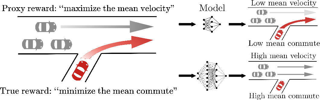
Economics has Goodhart’s law: “When a measure becomes a target, it ceases to be a good measure.” In reinforcement learning, this is particularly deadly. What we truly want is $R^*$ (the objective in the human mind), but in engineering we can only write or learn a proxy reward $R$. As long as $R \neq R^*$, optimization amplifies the gap between them.

This is not a purely theoretical concern; it appears repeatedly in practice. A classic example is the game Coast Runners^[12]. The objective is to win a boat race, and the reward is designed as “score points by collecting green blocks.” The agent learns to drive in circles in a corner, repeatedly collecting the same block, and never finishes the race. Its score far exceeds that of a “normal racing” strategy, yet it never completes the intended task. Similarly, in a bicycle simulator where the reward measures only “closeness to target,” the agent may learn to circle near the target: always close, never arriving.

The same issue recurs in Minecraft experiments. Researchers designed dense intermediate rewards to encourage the agent to gather resources and craft tools in order to complete a complex task. The agent learned to survive safely and continuously collect resources, but almost never attempted to complete the final goal, because “survive + collect” already yields high reward. Dense rewards turned “means” into “ends”^[4:1].

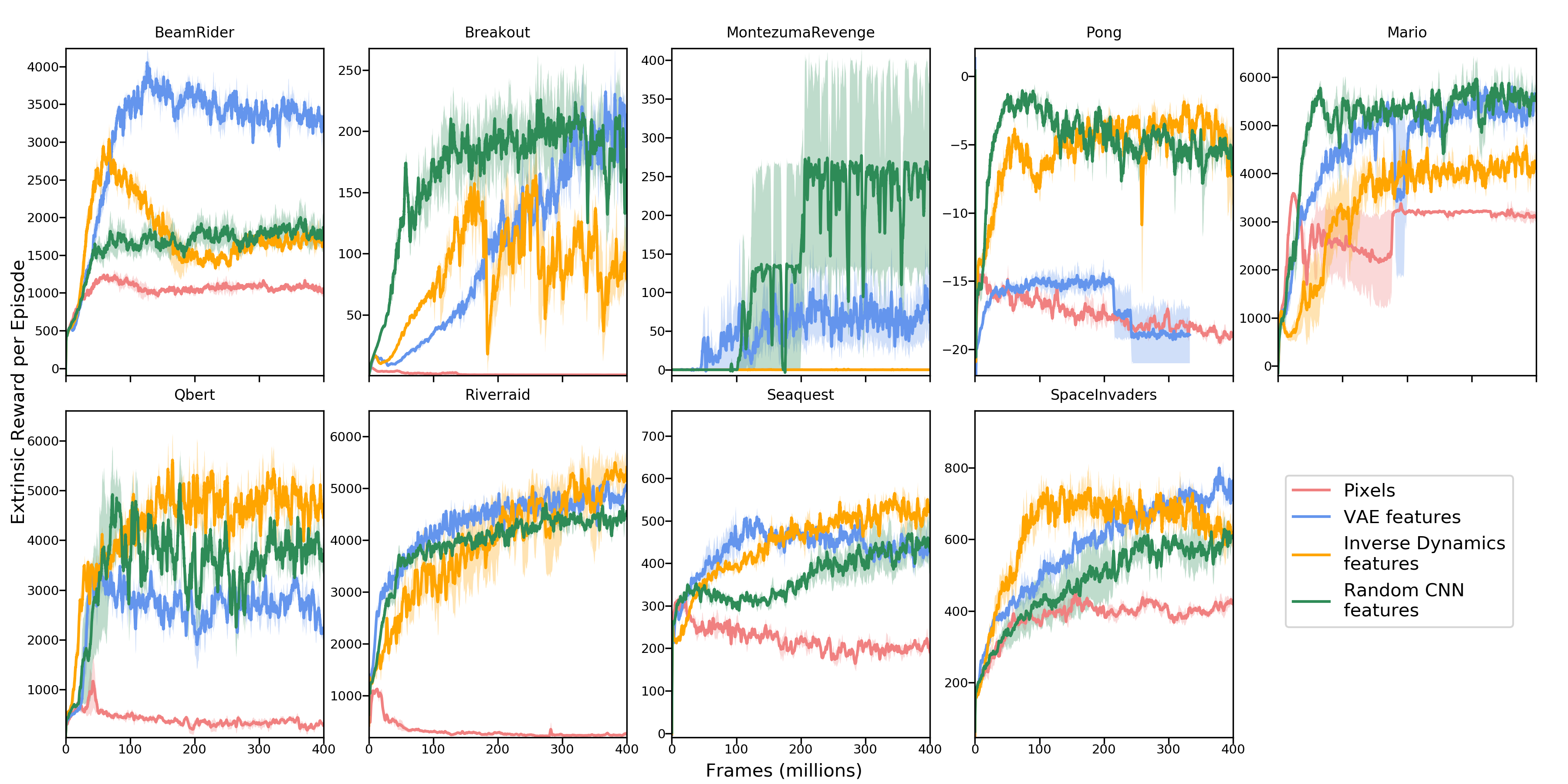
Curiosity-driven methods can have similar side effects. The Intrinsic Curiosity Module (ICM) proposed by Pathak et al. uses forward-model prediction error as an intrinsic reward: the agent is “curious” about unexpected transitions^[9:1]. In sparse-reward environments, this greatly improves exploration, e.g., discovering new rooms in Montezuma’s Revenge. But it also introduces a failure mode: if the environment contains a TV that constantly plays random frames, the agent will be attracted there forever, because randomness yields permanently high prediction error. This is the famous Noisy-TV Problem^[10:1]: intrinsic reward itself can become an exploitable target.

Consider CartPole again from Chapter 1. A common reward gives $+1$ for each step the pole does not fall, formulating the task as “live as long as possible.” This direction is broadly correct, but it also encodes a design choice: we do not explicitly reward “keep the pole angle close to vertical,” nor penalize “the cart drifts too far from center.” If we change it to

$$R(s,a)=1-c_1|\theta|-c_2|x|,$$

where $\theta$ is the pole-angle deviation and $x$ is the cart-position deviation, learning may speed up. But the magnitudes of $c_1$ and $c_2$ change behavior: if the position penalty is too strong, the agent becomes overly conservative and would rather let the pole tilt than move away from center; if the angle penalty is too strong, it may push the cart toward the boundary just to straighten the pole.

These examples show different degrees of misspecification. Pan et al. categorize reward misspecification into three types^[13]:

• Wrong weights: the direction is correct, but the relative importance across dimensions is wrong. In CartPole, choosing $c_1$ and $c_2$ is a weight issue.
• Wrong ontology: the measured dimension is wrong. Coast Runners uses “collect green blocks” to measure “racing performance,” which is the wrong object of measurement.
• Wrong scope: the reward covers only part of the scenarios and misses boundary cases. A reward that works in the training environment may fail completely in a new environment.

The same issues appear in LLM preference training. RLHF uses a reward model to score responses, but that reward model can learn superficial correlations such as “longer and more polite answers score higher.” After optimization, the language model starts to pile on boilerplate: the score is high, but the answer is not necessarily more accurate^[3:1]. More subtly, RLHF may teach the model to write in a way that “looks right but is actually wrong”: human evaluators are easier to persuade, and the error rate can increase^[14].

The essence of these phenomena is the same: the proxy reward $R$ is an imperfect approximation of the true intent $R^*$, and optimization amplifies the imperfect parts. The stronger the model and the more thorough the optimization, the more visible the gap between $R$ and $R^*$ becomes.

Figure 1: Read this figure from left to right. The red car on the left truly wants to “reduce average commute time,” but the engineer’s proxy reward is “increase average speed,” which pushes the agent toward behaviors that look faster but actually worsen the commute. The top and bottom rows on the right represent different model sizes: the stronger the model, the more likely it is to exploit loopholes in the proxy reward. This corresponds to the three misspecification types in the text: wrong weights, wrong ontology, and wrong scope. Source: Pan et al. (2022), The Effects of Reward Misspecification

Preference Learning and Reward Models

In many tasks, reward misspecification is not because the reward was written imprecisely, but because it cannot be written at all. How should we score a response? How do we judge whether a robot motion looks “natural”? These objectives are hard to encode as $R(s,a)$, but humans can often compare which of two outcomes is better.

So we can reformulate reward design as a preference-learning problem. Given the same prompt, let a model produce two answers $y_A$ and $y_B$, and ask humans which one they prefer. A reward model $r_\phi(x,y)$ learns to predict this preference, where $x$ is the input prompt, $y$ is the model output, and $\phi$ are the reward-model parameters.

Figure 2: RLHF reframes “we cannot write the reward” into “we can learn the reward from preferences.” Step 1 performs supervised fine-tuning on demonstration answers so the model can answer at all. Step 2 asks humans to rank multiple answers and trains a reward model from those rankings. Step 3 uses the reward model as a scorer and continues optimizing the language model with PPO. Note that the reward model is not the true human intent itself; it is a proxy learned from preference data. Source: OpenAI Aligning language models to follow instructions

A common training objective encourages preferred answers to receive higher scores. For example, if humans prefer $y_A$ over $y_B$, we want

$$r_\phi(x,y_A)>r_\phi(x,y_B).$$

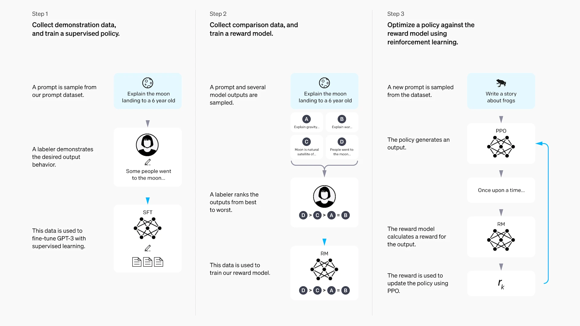
The point is not that “humans wrote down the reward formula,” but that “humans, by comparing samples, indirectly teach the model what outputs are more reward-worthy.” Concretely, the training data consists of preference pairs $(x, y_w, y_l)$, where $y_w$ is the chosen answer (win) and $y_l$ is the rejected answer (lose). The reward model is typically trained with a Bradley-Terry objective: maximize the probability that the chosen answer’s score exceeds the rejected answer’s score. After training, $r_\phi$ can output a scalar score for any $(x, y)$, and subsequent policy optimization (often PPO) treats $r_\phi$ as the reward signal.

This pipeline changes “defining rewards” from “writing formulas” into “collect preference data + train a model,” greatly increasing expressiveness. But the reward model itself is still a proxy reward, and it still faces the problem $R \neq R^*$.

Reward Model Overoptimization

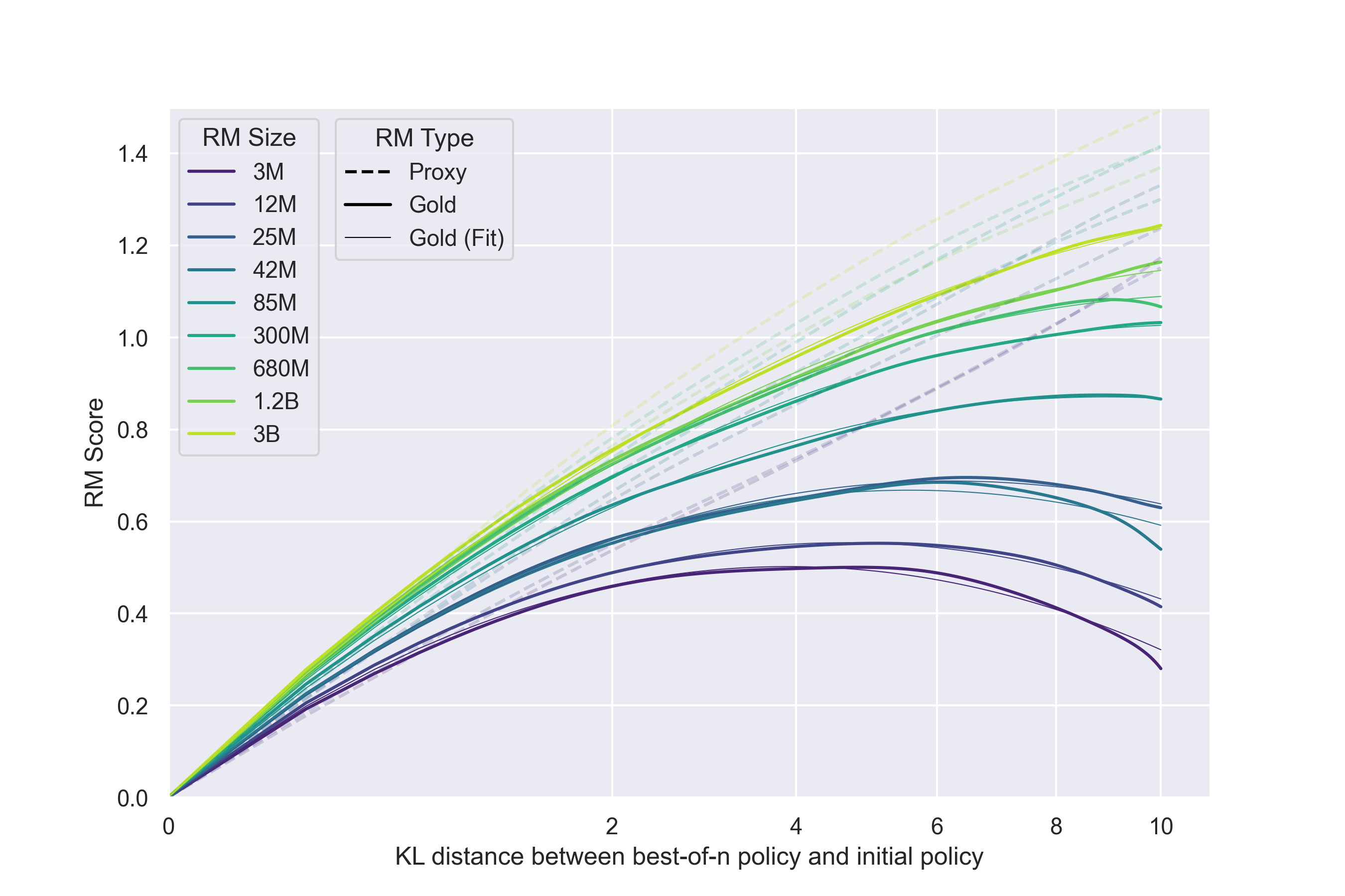
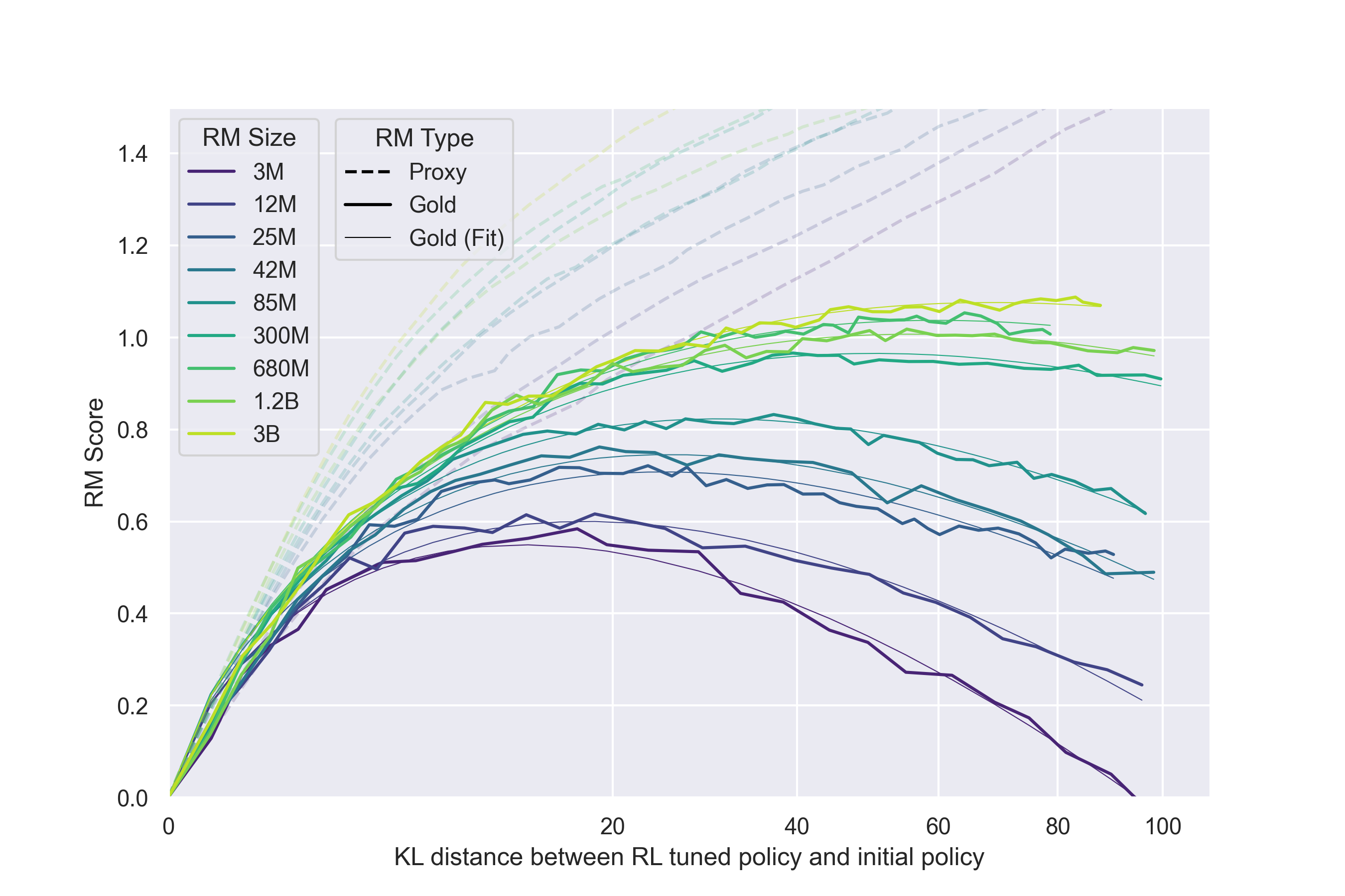
Gao et al. studied this problem systematically^[15]. They used a large model (6B parameters) as a “gold” reward, trained smaller models (3M to 3B parameters) as proxy reward models, and then used reinforcement learning to optimize the proxy reward. They observed a clear pattern: as optimization proceeds, the proxy reward continues to rise, but the gold reward rises only up to a peak and then declines.

The intuition is not hard. A reward model is trained from limited preference data. It learns not only “what answers are truly better,” but also many statistical correlations in the dataset, such as “longer answers tend to be chosen,” or “certain polite phrases are correlated with preference.” Once optimized, the policy becomes increasingly good at exploiting these correlations: it writes longer responses and adds more polite boilerplate to obtain higher proxy reward. But the connection between those behaviors and “truly helpful” gets weaker, and can even become negatively correlated.

In other words, optimization finds loopholes in the reward model, not the true human preference. This is Goodhart’s law manifesting directly in RLHF.

Figure 3: Both plots show the same phenomenon. The x-axis represents stronger optimization; the y-axis is reward score. The colored curve is the optimized proxy reward, and the dashed gray curve is the gold reward that is closer to true preference. At first both rise, meaning optimization helps; after the peak, the proxy reward keeps rising while the gold reward declines, meaning the model is starting to exploit loopholes in the proxy rather than becoming genuinely better. The upper plot uses Best-of-N sampling; the lower plot uses RL optimization. Source: Gao et al. (2023), Scaling Laws for Reward Model Overoptimization

Process Reward Models

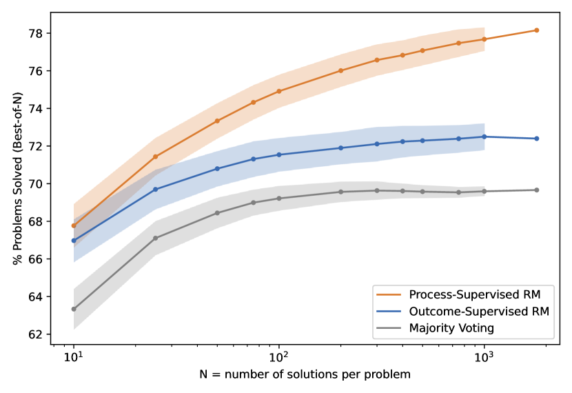
Standard reward models score only the overall quality of the final answer; this is an Outcome Reward Model (ORM). But in reasoning tasks, a correct final answer does not imply a correct reasoning process: the model may skip steps, guess correctly, or even use a flawed process that happens to arrive at the right result.

The idea of a Process Reward Model (PRM) is to score not only the final outcome, but also each step in a reasoning chain. Each step receives a score indicating whether “this step is correct” and whether it is “moving in the right direction.” This turns a sparse final reward into denser step-level rewards, providing richer learning signals and making it easier to localize where reasoning went wrong.

The cost of process rewards is labeling effort: humans must evaluate the quality of every step in a reasoning chain, which is much more time-consuming than judging only the final answer. Some work therefore uses trained models to automatically generate step labels and reduce reliance on manual annotation.

Figure 4: This figure compares ORM (score only the final answer) and PRM (verify each reasoning step). The x-axis selects an answer from more candidate solutions (further right means more candidates); the y-axis is the probability that the selected answer is correct. PRM curves are higher, meaning: when the model generates many reasoning chains, step-by-step verification is better at selecting genuinely reliable solutions than scoring only the final outcome. This matches the text’s conclusion: process rewards break sparse final feedback into more localizable step feedback. Source: Lightman et al. (2023), Let’s Verify Step by Step

AI Feedback

Collecting human preference data is one of the most expensive steps in RLHF. A natural idea is: can AI provide preferences? This is the core idea of RLAIF (Reinforcement Learning from AI Feedback). Constitutional AI is a representative approach: the AI model generates two candidate answers; another AI judge, guided by a predefined “constitution” (a set of behavioral principles), decides which answer is more compliant; the resulting AI-generated preference data is then used to train a reward model.

RLAIF substantially reduces labeling cost, but introduces a new question: are AI preferences reliable? If AI judgments diverge from true human preferences, then the problem $R \neq R^*$ is merely shifted from “human feedback” to “AI feedback.”

Bypassing Reward Models: GRPO

All methods above rely on an explicit reward model. But training a reward model is itself a source of $R \neq R^*$. GRPO (Group Relative Policy Optimization) tries to bypass this: for the same problem, generate a group of answers (e.g., 8), rank them using some rule (e.g., correctness checks or another model’s judgment), and then use within-group relative ranking as the reward signal to update the policy directly.

The key difference is that GRPO does not require training a separate reward model. The reward signal comes from relative comparisons within the current batch rather than a fixed scoring function. This works especially well for tasks like mathematical reasoning where answers are verifiable: correctness can be checked automatically without human judgment. Chapter 9 will describe GRPO’s mechanism and implementation in detail.

Summary

These methods share the goal of mitigating the fundamental tension $R \neq R^*$, but from different angles:

Method	Core Idea	What It Mitigates	New Risk Introduced
ORM	learn an overall reward from preferences	hand-written reward is hard	overoptimization, superficial correlations
PRM	score each step separately	outcome reward is too sparse	high labeling cost
RLAIF	replace human labels with AI	human labeling cost	whether AI preferences are reliable
GRPO	within-group ranking, no reward model	reward model’s own bias	requires a verifiable ranking rule

No method can completely eliminate the problem $R \neq R^*$. Reward design remains one of the hardest and most important parts of reinforcement learning.

A reward function is not “better” simply because it is more complex, nor because it is denser. The real question is whether it expresses the task’s key preferences clearly, without opening obvious loopholes. When designing rewards, it helps to check a few guiding questions: when the agent gets a high reward, would a human truly say the task is done well? Can the agent farm reward by repeating a local behavior? Are intermediate rewards helping learning, or have they already changed the final objective? Is the reward signal too sparse, making it hard for the algorithm to discover successful trajectories? For LLMs or complex robot tasks, are hand-written rules insufficient so we need to learn rewards from preferences? If we use a reward model, could overoptimization decouple the proxy reward from true preferences?

There is no universal answer. Control tasks like CartPole can start from survival time and angle deviation; grid worlds can start from terminal reward and step cost; LLM tasks often require preference data and reward models. Scenarios differ, reward expressions differ, but the underlying logic is the same: reward defines the direction of optimization, and that direction is almost never perfectly aligned with true intent. Good reward design is about finding a workable balance between alignment and feasibility.

Summary

This section discussed how reward functions determine the objective in reinforcement learning.

1. Reward is a scalar signal in the MDP that defines the task objective; return is the discounted sum of future rewards. Algorithms maximize return, so the reward specification directly determines learned behavior. Reward is one-step feedback; value is an estimate of long-term return. A value function depends on the reward definition and cannot be interpreted independently.
2. Sparse rewards are closer to the true objective but provide weak learning signals. Dense rewards can accelerate learning but often introduce the designer’s preferences and errors. Delayed rewards make credit assignment harder.
3. Reward shaping (PBRS) provides a theoretical guarantee: if the shaping term has the potential form $F(s,s') = \gamma\Phi(s') - \Phi(s)$, the optimal policy is unchanged. This is an effective tool for adding dense signals without changing the objective.
4. Multi-objective reinforcement learning works with reward vectors rather than scalars. Linear weighting is simple but can only find solutions in convex regions; Pareto frontiers and conditional policies cover a richer trade-off space; constrained optimization enforces safety requirements as hard boundaries.
5. Goodhart’s law captures the fundamental difficulty of reward design: proxy reward $R$ is almost never equal to true intent $R^*$, and optimization amplifies the gap. Wrong weights, wrong ontology, and wrong scope are common misspecification types.
6. When hand-written rewards fail, we can learn reward models from human preferences. But reward models are still proxy rewards, and overoptimization can reduce true preference. Process reward models and GRPO are newer methods that try to mitigate the issue from different directions.

The next section will put MDPs, returns, value functions, Bellman equations, algorithm families, and reward design back onto the same map. You will see that the concepts that seemed scattered throughout this chapter are all organized around the same question: how do we formulate a sequential decision-making problem in a way that is learnable, optimizable, and as faithful as possible to true intent?

← Previous: Where Does the Data Come From? | Next: Chapter Summary

References

---

1. Ng, A. Y., Harada, D., & Russell, S. (1999). Policy invariance under reward transformations: Theory and application to reward shaping. ICML. ↩︎

2. Xu, J., Tian, Y., Ma, P., Rus, D., Sueda, S., & Matusik, W. (2020). Prediction-guided multi-objective reinforcement learning for continuous robot control. ICML. ↩︎

3. Ouyang, L., Wu, J., Jiang, X., Almeida, D., Wainwright, C. L., Mishkin, P., Zhang, C., Agarwal, S., Slama, K., Ray, A., Schulman, J., Hilton, J., Kelton, F., Miller, L., Simens, M., Askell, A., Welinder, P., Christiano, P. F., Leike, J., & Lowe, R. (2022). Training language models to follow instructions with human feedback. NeurIPS. ↩︎ ↩︎

4. Amin, S., et al. (2024). Comprehensive overview of reward engineering and shaping in advancing reinforcement learning applications. arXiv preprint arXiv:2408.10215. ↩︎ ↩︎

5. Nair, S., Savarese, S., & Finn, C. (2020). Goal-aware prediction: Learning to model what matters. CoRL. ↩︎

6. Ho, J., & Ermon, S. (2016). Generative adversarial imitation learning. NeurIPS. ↩︎

7. Andrychowicz, M., Wolski, F., Ray, A., Schneider, J., Fong, R., Welinder, P., McGrew, B., Tobin, J., Pieter Abbeel, O., & Zaremba, W. (2017). Hindsight experience replay. NeurIPS. ↩︎

8. Achiam, J., Held, D., Tamar, A., & Abbeel, P. (2017). Constrained policy optimization. ICML. ↩︎

9. Pathak, D., Agrawal, P., Efros, A. A., & Darrell, T. (2017). Curiosity-driven exploration by self-supervised prediction. ICML. ↩︎ ↩︎

10. Burda, Y., Edwards, H., Pathak, D., Storkey, A., Darrell, T., & Efros, A. A. (2018). Large-scale study of curiosity-driven learning. ICLR. ↩︎ ↩︎

11. van Hasselt, H., Hessel, M., & Aslanides, J. (2016). When using function approximation, a simpler target often yields better results. Deep Reinforcement Learning Workshop, NeurIPS. ↩︎ ↩︎

12. Amodei, D., Olah, C., Steinhardt, J., Christiano, P., Schulman, J., & Mané, D. (2016). Concrete problems in AI safety. arXiv preprint arXiv:1606.06565. ↩︎

13. Pan, A., Bhat, M., Shern, C., Phadnis, S., Guss, W., & Amodei, D. (2022). The effects of reward misspecification: Mapping and mitigating misaligned models. arXiv preprint arXiv:2201.03544. ↩︎

14. Wen, J., Zhong, R., Khan, A., Jørgensen, E., Wu, J., Tran, D., Peng, Z., Peng, B., & He, H. (2024). Language models learn to mislead humans via RLHF. arXiv preprint arXiv:2409.12822. ↩︎

15. Gao, L., Schulman, J., & Hilton, J. (2022). Scaling laws for reward model overoptimization. ICML. ↩︎