12.2 Model-Based RL: From Model-Free to Model-Based

In embodied intelligence, the real world is not a Gym environment that can be reset() indefinitely. If a robotic arm misses a grasp, it may hit the table. If a quadruped falls, a person may have to pick it up. Autonomous driving certainly cannot explore boundary conditions through real accidents. Therefore, one of the central questions in embodied RL is: can we do less trial and error in the real world, and more reasoning inside a "mental world"?

This is the starting point of Model-Based RL (MBRL). The agent first learns a model of the environment, then uses that model for planning, for generating imagined trajectories, or for assisting policy updates. Compared with model-free methods, MBRL does not only try to learn "what should I do in this state?" It also tries to learn "if I do this, how will the world change?"

Figure 1: A roadmap of world models in deep learning. Source: Ding et al., "Understanding World or Predicting Future? A Comprehensive Survey of World Models", Fig. 1[^worldmodelsurvey].

Reading path

If the formulas later feel difficult, first return to the beginning of the article or read the intuitive version. The main text follows the order "meaning of symbols -> formula -> plain-English explanation." On the first pass, you do not need to memorize every symbol.

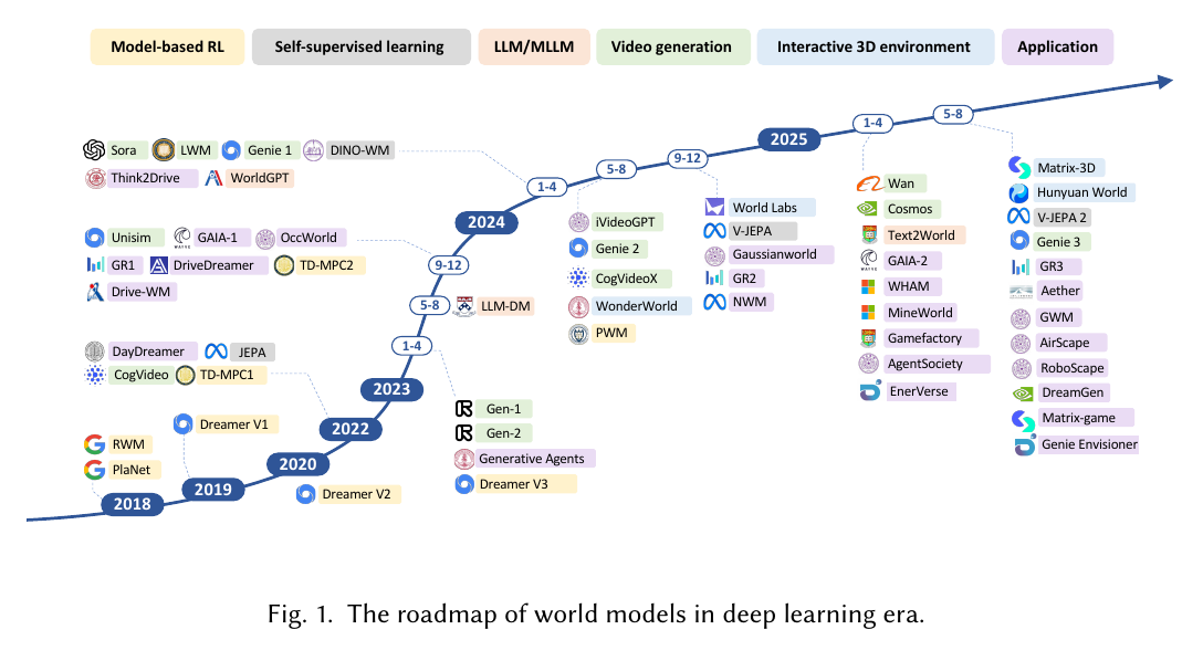
From Surveys: There Is More Than One Kind of World Model

Recent surveys remind us that "world model" is no longer a small concept that belongs only to reinforcement learning. Ding et al. summarize world models through two core functions: one is understanding the world, meaning the construction of internal representations that capture world mechanisms; the other is predicting future dynamics, meaning the prediction of future states to support simulation, planning, and decision-making^[1]. The MBRL discussed in this section mainly falls into the second category, but it often borrows representation-learning capabilities from the first.

From the perspective of embodied intelligence, world models can also be divided along three axes^[2]:

Dimension	Typical question	Meaning for MBRL
Function	Does it serve a particular control task, or general simulation?	Determines whether the model should directly predict reward/value
Temporal modeling	Step-by-step autoregressive rollout, or parallel prediction?	Determines whether long-horizon error accumulation is likely
Spatial representation	Low-dimensional states, tokens, BEV/voxels, 3D representations	Determines whether the model can handle vision, contact, and geometric constraints
Coupling with decision-making	Does it only generate the future, or directly participate in planning?	Determines whether it is closer to a video model, a simulator, or a controller

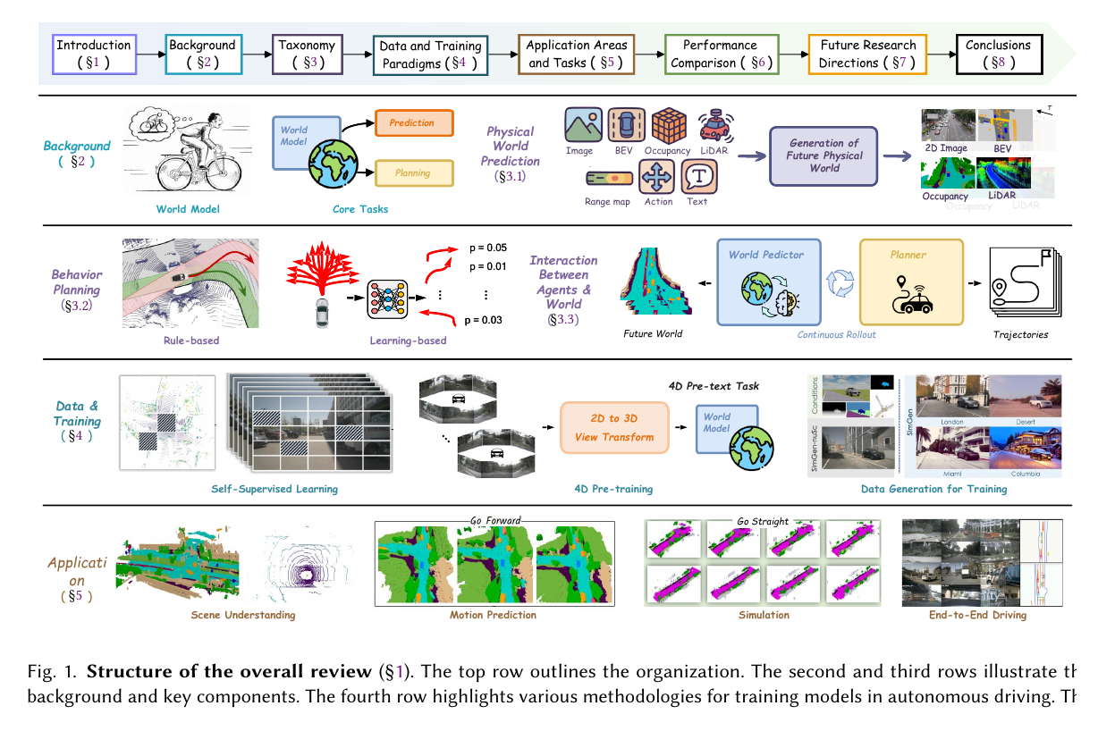
Surveys of world models for autonomous driving also give a more engineering-oriented taxonomy: world models can be used to generate future physical worlds, to plan agent behavior, or to place prediction and planning inside the same interactive loop^[3]. This is very close to embodied robotics: a robot must both "see possible futures" and "choose a future it can reach safely."

Therefore, this article uses a convergent definition: in MBRL, a world model is a model that compresses the current state, action, and history into a predictable representation, and supports future rollout, planning search, or policy training. It may be a low-dimensional dynamics model, a latent-space model like Dreamer, an implicit model used only for search as in MuZero, or it may borrow ideas from broader world models such as video generation, JEPA representations, and occupancy prediction in autonomous driving.

Model-Free vs Model-Based

Most algorithms covered so far in this book, from DQN, PPO, and SAC to DPO and GRPO, belong to Model-Free RL. The agent does not explicitly learn environment dynamics. It optimizes a value function or policy only through real or simulated interaction.

Read It Intuitively First

For the moment, put the formulas aside and remember only these three sentences:

• Model-Free: do not learn "how the world changes"; directly learn "what I should do" from real interaction.
• Model-Based: first learn an approximate model of "how the world changes," then use it for planning or imagined experience.
• Key difference: the issue is not whether environment transitions exist, but whether the agent learns those transition rules as a callable model.

If you only want the main thread, read this paragraph and the table below first. The formulas will feel much smoother after you have run the minimal practice example.

Mathematically, model-free does not mean "there is no environment transition." It means we do not explicitly learn that transition model. First, align the notation:

Symbol	How to understand it first
$s_t$	The state at step $t$, such as robot joint angles, velocities, or camera features
$a_t$	The action at step $t$, such as torque, velocity command, or gripper open/close
$r_t$	The reward received at step $t$
$\pi_\theta$	The policy, the model that decides how to choose actions after seeing a state
$p$	The true transition law of the environment
$\hat{p}_\phi$	The world model learned by the agent, with parameters $\phi$
$\gamma$	The discount factor; later rewards receive smaller weight

In the real environment, a transition law always exists:

$$p(s_{t+1}\mid s_t,a_t)$$

This formula says: if the current state is $s_t$ and the agent takes action $a_t$, the real environment produces the next state $s_{t+1}$. Model-free methods also experience this transition; they simply do not learn it as a callable model.

One interaction trajectory can be written as:

$$\tau=(s_0,a_0,r_0,s_1,\ldots),\qquad s_{t+1}\sim p(\cdot\mid s_t,a_t),\quad a_t\sim \pi_\theta(\cdot\mid s_t)$$

In plain language: the agent first observes $s_t$, the policy $\pi_\theta$ samples an action $a_t$, and the real environment $p$ returns the next state $s_{t+1}$ and reward $r_t$. Here, $\tau$ is the whole recorded segment of experience.

Model-free RL directly optimizes "how much score can I get on average":

$$J_{\text{MF}}(\theta) = \mathbb{E}_{\tau\sim p,\pi_\theta} \left[ \sum_{t=0}^{\infty}\gamma^t r_t \right]$$

Read this formula in three layers. The inner $\sum_t \gamma^t r_t$ is the total return of one trajectory; $\gamma^t$ gives less weight to rewards farther in the future; the outer expectation means both the environment and the policy may be random, so we look at the average score over many trajectories. Training a model-free policy means making $J_{\text{MF}}(\theta)$ larger.

If we follow the policy-gradient route, such as REINFORCE, A2C, or PPO, the core update is:

$$\nabla_\theta J_{\text{MF}}(\theta) = \mathbb{E}_{\tau\sim p,\pi_\theta} \left[ \sum_t \nabla_\theta \log \pi_\theta(a_t\mid s_t)\,\hat{A}_t \right]$$

The plain-English version is: if an action produces a result better than average, increase the probability that the policy chooses it in the future; if it produces a worse result, decrease that probability. $\log \pi_\theta(a_t\mid s_t)$ is the log probability that the policy chooses $a_t$ under $s_t$, and $\hat{A}_t$ measures how much better this action is than the reference level.

If we follow the value-function route, such as DQN, SAC, or TD3, the core step is to construct a TD target:

$$y_t = r_t+\gamma(1-d_t)\max_{a'}Q_{\bar{\theta}}(s_{t+1},a')$$

Here, $y_t$ is a temporary answer for the critic: the current reward $r_t$, plus the value that can still be obtained from the next state. If the episode has ended, $d_t=1$, and the later term is removed by $(1-d_t)$.

The critic loss is:

$$\mathcal{L}_{Q}(\theta) = \mathbb{E}_{(s,a,r,s',d)\sim\mathcal{D}} \left[ \big(Q_\theta(s,a)-y_t\big)^2 \right]$$

Its meaning is simple: the current critic predicts $Q_\theta(s,a)$, the temporary answer is $y_t$, and training makes the two as close as possible. The most important detail is the data source: $s_{t+1}$ comes from the real environment or from a replay buffer recorded by a simulator. It is not generated by a neural-network world model.

MBRL adds one more layer: a "world model." It not only optimizes a policy or value function, but also explicitly learns an approximate model of the environment:

$$\hat{p}_\phi(s_{t+1}, r_t \mid s_t, a_t)$$

The $p$ without a hat denotes the true environmental law; $\hat{p}_\phi$ with a hat denotes "the approximate version I learned from data." It may predict the next state, reward, termination probability, or, in more modern methods, future representations in latent space.

With a world model, the agent can first try action sequences inside the model, then choose the one predicted to be best:

$$a_{0:H-1}^{*} = \arg\max_{a_{0:H-1}} \sum_{h=0}^{H-1} \gamma^h\hat{r}_\phi(\hat{s}_{t+h},a_{t+h})$$

In this formula, $\arg\max$ means "find the candidate action sequence with the highest score"; $H$ is the lookahead horizon; the hats on $\hat{s}$ and $\hat{r}$ indicate that these states and rewards come from the world model. MPC usually does not execute the whole sequence at once. It executes only the first action $a_0^\*$, observes the new real state, and plans again.

The model can also generate imagined experience through rollout and use it to update the policy or value function:

$$\hat{s}_{t+h+1},\hat{r}_{t+h} \sim \hat{p}_\phi(\cdot\mid \hat{s}_{t+h},a_{t+h})$$

So the key mathematical difference is this: model-free learning signals come from real sampled next_state; model-based methods first learn a world_model, then use imagined states and imagined rewards predicted by the model for planning or training.

One-Table Summary

Dimension	Model-Free RL	Model-Based RL
Core idea	Directly learn a policy or value function	First learn a world model, then use it for planning or policy training
Sample efficiency	Usually lower; requires many interactions	Usually higher; can reuse the model to generate imagined experience
Main risk	Trial-and-error is expensive; exploration is slow	Model errors are amplified by planning
Representative algorithms	DQN, PPO, SAC, DPO, GRPO	Dyna, PETS, PlaNet, MuZero, Dreamer
Suitable scenarios	Cheap interaction, sufficient simulation, clear goals	Expensive interaction, need to predict the future, need safe trial and error
"Mental simulation"	No explicit simulation	Yes; the agent can reason about the future inside the model

As an intuitive analogy, model-free RL is like a chess player who learns only through real games; model-based RL is like a chess player who can mentally look ahead several moves. The former learns from real feedback at every step; the latter first imagines several possible routes, then decides how to act.

When the formulas feel confusing

Return to read it intuitively first, or jump directly to minimal MBRL practice. After the code runs, the formulas above will feel more like names for parts of the code, rather than symbols to memorize from nowhere.

Mathematically: What Does a World Model Learn?

The most basic MBRL setup collects real interaction into a dataset:

$$\mathcal{D}=\{(s_t, a_t, r_t, s_{t+1}, d_t)\}_{t=1}^{N}$$

This formula is just a more formal way to write a replay buffer. Each item contains five things: the current state $s_t$, the action $a_t$, the reward $r_t$, the next state $s_{t+1}$, and the termination flag $d_t$.

What the world model must learn is "given the current state and action, predict what will happen next":

$$\hat{p}_\phi(s_{t+1}, r_t, d_t \mid s_t, a_t)$$

The input is $(s_t,a_t)$, and the output is the next state, reward, and whether the episode ends. In code, this is world_model(state, action) -> next_state, reward, done. Different algorithms produce different output formats, but the core question is always the same: if I act like this now, what will the world do next?

If the state dimension is low, for example joint angles, velocities, and contact information in MuJoCo, a common approach is to predict the state difference:

$$\Delta s_t=s_{t+1}-s_t,\qquad \widehat{\Delta s_t}=f_\phi(s_t,a_t)$$

Why predict the difference? In many physical systems, the next state usually does not jump to a distant place out of nowhere. It changes near the current state. Learning the "amount of change" is often easier than learning the full $s_{t+1}$ directly. For example, if the current position is 2.0 and the next position is 2.1, the model only needs to learn "increase by 0.1."

A deterministic model can be trained with mean squared error:

$$\mathcal{L}_{\text{det}}(\phi) =\mathbb{E}_{\mathcal{D}}\left[ \|\Delta s_t-f_\phi(s_t,a_t)\|_2^2 +\lambda_r(r_t-\hat{r}_\phi(s_t,a_t))^2 \right]$$

This loss has two terms. The first makes the model's predicted state change $f_\phi(s_t,a_t)$ close to the true change $\Delta s_t$; the second makes the predicted reward $\hat{r}_\phi(s_t,a_t)$ close to the true reward $r_t$. $\lambda_r$ is a weight controlling how important reward prediction error is in the total loss.

Minimal Practice: Deterministic World Model + Random-Shooting MPC

For a first implementation, you do not need to start with PETS. A minimal MBRL practice can use a deterministic one-step dynamics model, then use the simplest random shooting method for MPC. This version is simple, but it already contains the full MBRL loop: collect real interaction data, train a world model, try many action sequences inside the model, and execute only the first action of the best sequence in the real environment.

We can use a one-dimensional point-mass environment that does not depend on Gym:

$$s_t=[x_t,v_t],\qquad a_t\in[-1,1]$$

The state has only two numbers: position $x_t$ and velocity $v_t$. The action $a_t$ can be understood as the force pushing left or right. It is limited to $[-1,1]$ to prevent actions from becoming unbounded.

$$v_{t+1}=0.95v_t+0.15\tanh(a_t),\qquad x_{t+1}=x_t+v_{t+1}$$

These two lines are the "true physics" of this small world. The next velocity is determined by the old velocity and the current action. $0.95v_t$ means the velocity is preserved but slightly decays, while $0.15\tanh(a_t)$ means the action changes the velocity. The position is then updated using the new velocity.

The reward asks the cart to return as close as possible to $x=0$, while avoiding high velocity and overly large actions:

$$r_t=-(x_{t+1}^2+0.1v_{t+1}^2+0.001a_t^2)$$

The negative sign is important. The larger the expression inside the parentheses, the farther the position is, the larger the velocity is, and the stronger the action is. After adding the negative sign, being closer to 0, smoother, and using smaller actions gives a higher reward.

The world model only needs to predict three things:

$$[\widehat{\Delta x_t},\widehat{\Delta v_t},\hat r_t] =f_\phi([x_t,v_t],a_t)$$

That is, after seeing the current position, velocity, and action, the model predicts "how much the position will change, how much the velocity will change, and what reward this step will receive." Adding the predicted difference to the current state gives the next state imagined by the model.

During planning, sample $M$ action sequences at random and roll them forward for $H$ steps in the model:

$$a_{0:H-1}^{*} = \arg\max_{a_{0:H-1}^{(j)},\,j=1,\ldots,M} \sum_{h=0}^{H-1}\gamma^h\hat r_{t+h}^{(j)}$$

Read this formula as a procedure. First randomly generate $M$ candidate action sequences. The $j$-th sequence is rolled forward for $H$ steps in the model, producing a sequence of predicted rewards $\hat r_{t+h}^{(j)}$. Sum these rewards, and choose the sequence with the highest total score. Finally, execute only $a_0^\*$, observe the new real state, and plan again. This is the minimal version of model predictive control.

The full script is in minimal_mbrl_point_mass.py, and can be run directly:

python docs/chapter12_future_trends/embodied-intelligence/model-based-rl/snippets/minimal_mbrl_point_mass.py

A typical result shows the random policy pushing the system farther away, while MBRL with MPC can pull the state back near the origin:

one_step_model_mse=0.013716
random_policy_return=-2246.07, final_state=[8.50, -0.25]
mbrl_mpc_return=-18.76, final_state=[0.17, 0.07]

The core code is:

# 1. The real environment is used only to collect data and execute final actions
state = env_reset()
action = torch.empty(1).uniform_(-1.0, 1.0)
next_state, reward = env_step(state, action)

# 2. The world model learns next_state - state and reward
target = torch.cat([next_state - state, reward.unsqueeze(-1)], dim=-1)
pred = model(state, action)
model_loss = ((pred - target) ** 2).mean()

# 3. MPC tries many action sequences inside the model
action_sequences = torch.empty(num_samples, horizon, 1).uniform_(-1.0, 1.0)
scores = score_action_sequences(model, state, action_sequences)
real_action = action_sequences[scores.argmax(), 0]

# 4. Execute only the first action in the real environment, then observe and replan
next_state, reward = env_step(state, real_action)

The point of this exercise is not performance, but making the concept run end to end: model-free RL directly learns policy(state) -> action or Q(state, action); minimal MBRL first learns model(state, action) -> next_state, reward, then treats that model as a temporary simulator for selecting actions.

Why does the main text still cite PETS? Because the minimal version above assumes "the model prediction is a single deterministic value." But contact, friction, sensor noise, and occlusion in robotics are often not deterministic. When data is scarce, the model may also "not know that it does not know." The value of PETS^[4] is not that it is required for beginners, but that it places probabilistic dynamics models, model ensembles, uncertainty propagation, and MPC into one clear framework, making it a good example for understanding risk control in modern MBRL.

One key contribution of PETS is using a probabilistic dynamics model ensemble to express uncertainty:

$$p_{\phi_i}(\Delta s_t, r_t\mid s_t,a_t) =\mathcal{N}(\mu_{\phi_i}(x_t), \Sigma_{\phi_i}(x_t)), \qquad x_t=[s_t,a_t]$$

This differs from the deterministic model above. A deterministic model gives one answer: "I think the state will change this way." The probabilistic model in PETS gives a distribution: "I think the most likely change is $\mu$, but there is uncertainty of size $\Sigma$." The subscript $i$ denotes the $i$-th member of the ensemble.

The training objective is usually written as Gaussian negative log likelihood:

$$\mathcal{L}_{\text{nll}}(\phi_i) = \frac{1}{2}(y_t-\mu_{\phi_i})^\top\Sigma_{\phi_i}^{-1}(y_t-\mu_{\phi_i}) +\frac{1}{2}\log |\Sigma_{\phi_i}|, \qquad y_t=[\Delta s_t,r_t]$$

This loss can also be read in two parts. The first term is like a "weighted squared error": if the true target $y_t$ is far from the predicted mean $\mu_{\phi_i}$, the penalty is large; if the model itself predicts a large variance $\Sigma_{\phi_i}$, meaning it admits uncertainty, this error penalty is softened. The second term, $\log|\Sigma_{\phi_i}|$, penalizes making the variance infinitely large. Therefore, the model cannot avoid all mistakes by saying "I am very uncertain." It must balance prediction accuracy with honest uncertainty estimation.

Figure 2: PETS uses probabilistic dynamics models, trajectory propagation, and MPC for low-sample control. Source: Chua et al., "Deep Reinforcement Learning in a Handful of Trials using Probabilistic Dynamics Models", Fig. 1[^pets].

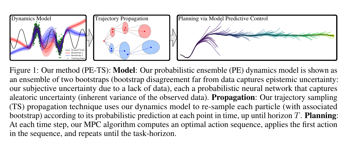
Two details are especially important here.

First, the model's output variance $\Sigma_{\phi_i}$ can describe aleatoric uncertainty, the randomness inherent in the environment; disagreement between different ensemble members can describe epistemic uncertainty, the "not knowing whether one knows" caused by insufficient data. For embodied robots, the second type is especially important: if several models strongly disagree about the consequence of an action, that region of state-action space is not reliable, and planning should be conservative.

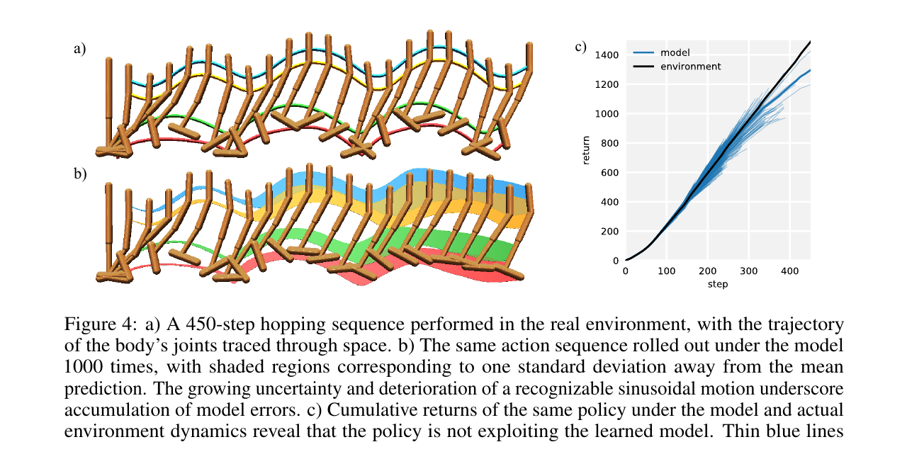
Second, the farther a world model rolls out, the more errors accumulate. Roughly speaking, if the one-step model error is $\epsilon_{\text{model}}$, then the $k$-step prediction error grows with $k$:

$$\epsilon_{t+k}\approx \mathcal{O}(k\epsilon_{\text{model}})$$

This formula is not meant to be memorized as a strict theorem. It says that being only slightly wrong for one step can become very wrong after many rollout steps. If step 1 is predicted incorrectly, the next prediction uses that incorrect state as input, and the error propagates along the rollout. This is why many successful MBRL systems do not blindly trust long imagination. PETS replans with MPC at every step, MBPO^[5] uses the model only for short rollouts, and Dreamer imagines the future in a compressed latent space; all of these reduce the risk of amplified model bias.

Advanced Code: Training a Probabilistic Dynamics Model

Below is a minimal PyTorch dynamics model. Real systems also use input normalization, model ensembles, early stopping, reward heads, and termination heads. Here we keep only the core mathematical correspondence.

import torch
import torch.nn as nn


class ProbabilisticDynamics(nn.Module):
    def __init__(self, state_dim: int, action_dim: int, hidden_dim: int = 256):
        super().__init__()
        out_dim = state_dim + 1  # delta_state + reward
        self.net = nn.Sequential(
            nn.Linear(state_dim + action_dim, hidden_dim),
            nn.SiLU(),
            nn.Linear(hidden_dim, hidden_dim),
            nn.SiLU(),
        )
        self.mu = nn.Linear(hidden_dim, out_dim)
        self.logvar = nn.Linear(hidden_dim, out_dim)

    def forward(self, state: torch.Tensor, action: torch.Tensor):
        h = self.net(torch.cat([state, action], dim=-1))
        mu = self.mu(h)
        logvar = self.logvar(h).clamp(-10.0, 2.0)
        return mu, logvar


def gaussian_nll(mu: torch.Tensor, logvar: torch.Tensor, target: torch.Tensor):
    inv_var = torch.exp(-logvar)
    return 0.5 * ((target - mu) ** 2 * inv_var + logvar).mean()


def train_step(model, optimizer, batch):
    state, action, reward, next_state = batch
    target = torch.cat([next_state - state, reward.unsqueeze(-1)], dim=-1)

    mu, logvar = model(state, action)
    loss = gaussian_nll(mu, logvar, target)

    optimizer.zero_grad()
    loss.backward()
    optimizer.step()
    return loss.item()

This code corresponds to the $\mathcal{L}_{\text{nll}}$ above: the model predicts not only the mean $\mu$, but also the uncertainty logvar in each dimension. During planning, we can sample multiple futures from this Gaussian distribution, or add uncertainty to the penalty term so that the robot avoids actions the model is not confident about.

Advanced Code: Using CEM for MPC Planning

After we have a model, the most direct control method is MPC: sample a batch of action sequences, evaluate their future returns with the model, keep elite sequences to update the distribution, and finally execute only the first action. The CEM (Cross-Entropy Method) below is a common planning skeleton used in PETS- and MPC-style methods.

@torch.no_grad()
def rollout_model(model, state, actions, discount=0.99):
    # actions: [num_samples, horizon, action_dim]
    num_samples, horizon, _ = actions.shape
    state = state.expand(num_samples, -1)
    returns = torch.zeros(num_samples, device=state.device)
    gamma = 1.0

    for t in range(horizon):
        mu, logvar = model(state, actions[:, t])
        pred = mu + torch.randn_like(mu) * torch.exp(0.5 * logvar)
        delta_state, reward = pred[:, :-1], pred[:, -1]
        state = state + delta_state
        returns = returns + gamma * reward
        gamma *= discount

    return returns


@torch.no_grad()
def cem_plan(model, state, action_dim, horizon=15, iters=5, samples=512, elites=64):
    mean = torch.zeros(horizon, action_dim, device=state.device)
    std = torch.ones_like(mean)

    for _ in range(iters):
        actions = mean + std * torch.randn(samples, horizon, action_dim, device=state.device)
        actions = actions.clamp(-1.0, 1.0)
        scores = rollout_model(model, state, actions)
        elite_actions = actions[scores.topk(elites).indices]
        mean = elite_actions.mean(dim=0)
        std = elite_actions.std(dim=0).clamp_min(1e-3)

    return mean[0].clamp(-1.0, 1.0)

Notice that this planner returns only mean[0], the current action. After executing it, the agent receives a new real observation and replans the next step. This receding-horizon closed loop is much more stable than trusting the model's prediction dozens of steps into the future all at once.

Three Ways to Use MBRL

MBRL is not a single algorithm. It is a family of paradigms that place a "model" inside the RL loop.

Figure 3: Dreamer separates learning latent-space dynamics, learning behavior in imagination, and acting in the real environment into three components. Source: Hafner et al., "Dream to Control", Fig. 3[^dreamer].

1. Use the Model to Generate Data: The Dyna Idea

Sutton's Dyna architecture from 1991^[6] can be seen as a classic starting point for MBRL: the agent learns a model from the real environment, then uses the model to generate extra experience and update the value function as if that experience were real.

This resembles "synthetic data" in today's large-model training: real data is expensive, model-generated data is cheap. But the problem is also similar: if generated data is biased, training amplifies the bias.

# Dyna-style core loop (pseudocode)
for step in range(num_steps):
    s, a, r, next_s = env.step(policy(s))
    replay.add(s, a, r, next_s)
    world_model.fit(replay)

    for _ in range(planning_steps):
        imagined_s, imagined_a = replay.sample_state_action()
        imagined_next_s, imagined_r = world_model.predict(imagined_s, imagined_a)
        value_fn.update(imagined_s, imagined_a, imagined_r, imagined_next_s)

MBPO can be viewed as a modern Dyna variant: real environment data first enters a replay buffer, the world model learns from that replay buffer, and then short rollouts branch from real states and are added to policy learning^[5:1]. Its lesson is very simple: the model can help, but do not let the model imagine for too long.

Figure 4: The MBPO paper shows the same action sequence gradually diverging between the real environment and the model rollout, illustrating how long rollouts amplify model error. Source: Janner et al., "When to Trust Your Model", Fig. 4[^mbpo].

2. Use the Model for Planning: MPC, MCTS, and MuZero

Another route does not necessarily use the model to train the policy directly. Instead, it uses the model to search forward at each decision step.

In continuous control, the common method is MPC (Model Predictive Control): at every step, use the model to predict the next $H$ steps, choose the action sequence with the highest cumulative reward, execute only the first step, then observe again and replan. This "recompute while walking" style is especially suitable for robotics, because the real world always deviates from prediction.

In board games and Atari, AlphaZero^[7] and MuZero^[8] use tree search. AlphaZero relies on known rules for MCTS; MuZero goes further: it does not need the true rules, but searches inside a learned latent-space model.

3. Dream in Latent Space: PlaNet, Dreamer, and TD-MPC

The pixel world is too complex. One robot camera frame may contain hundreds of thousands of dimensions. Directly predicting future pixels is expensive and easily distracted by irrelevant details. Therefore, modern MBRL often first compresses observations into a latent space, then predicts the future in that latent space.

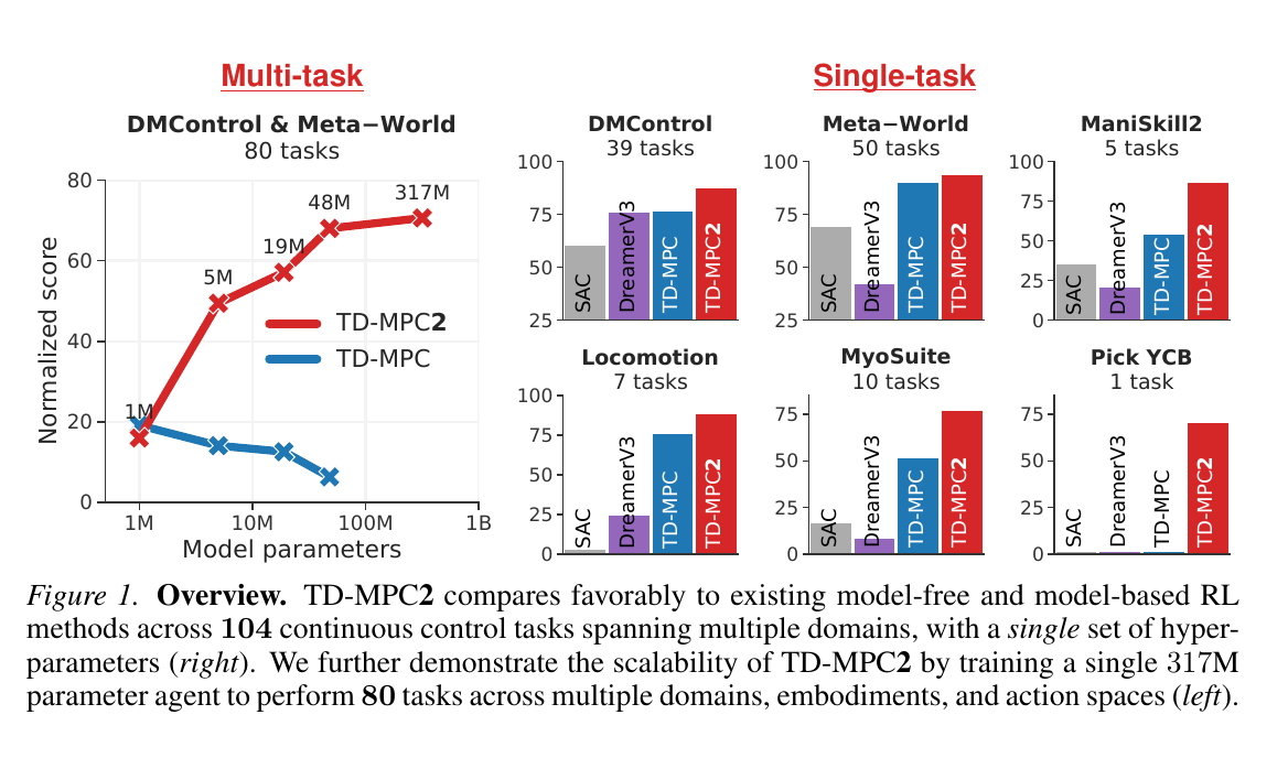
PlaNet^[9] systematically demonstrated the route of learning latent-space dynamics from pixels and then controlling through planning. The Dreamer series^[10][11] uses imagined trajectories for actor-critic training, allowing the policy to learn mainly in latent imagination. TD-MPC2^[12] further scales latent-space model predictive control to larger continuous-control tasks.

Intuitively, latent-space MBRL does not require the model to reconstruct every pixel. It only preserves information useful for control: robot pose, relative object locations, velocity trends, contact state, and so on.

Three Milestones

Figure 5: TD-MPC2 shows the scaling trend of modern latent-space world models in continuous control. Source: Hansen et al., "TD-MPC2", Fig. 1[^tdmpc2].

AlphaZero: Search with Known Rules

AlphaZero does not imitate human game records. It learns through self-play. It uses a neural network to evaluate positions and action priors, then uses MCTS for deep search^[7:1]. Here, the "model" is not learned neural-network dynamics, but the known rules of the board game.

This paradigm tells us that when the environment model is accurate enough, planning can significantly improve decision quality. The problem is that the physical world is not as clean as board-game rules.

MuZero: Planning Without Knowing the Rules

MuZero's breakthrough is that it does not need to know the true rules of the environment, yet it can learn an implicit model suitable for planning^[8:1]. This model does not try to reconstruct the full world. It only needs to support value prediction, reward prediction, and policy search.

This is very instructive for embodied intelligence: a robot may not need to learn "complete physics." It may only need dynamics representations that are sufficient for task decisions.

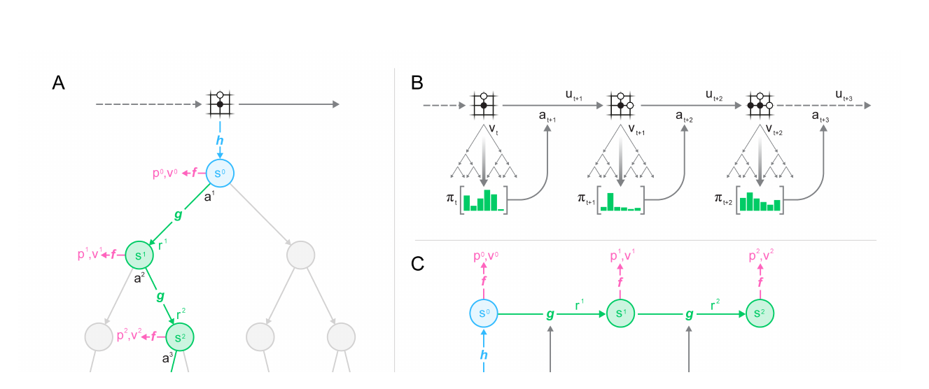
MuZero's model can be decomposed into three parts:

$$s_0=h_\theta(o_{1:t}),\qquad r_{k+1},s_{k+1}=g_\theta(s_k,a_k),\qquad p_k,v_k=f_\theta(s_k)$$

This formula can be split into three small models:

Module	Input	Output	Role
$h_\theta$	Observation history $o_{1:t}$	Initial latent state $s_0$	Compress real observations into a plannable state
$g_\theta$	Latent state $s_k$ and action $a_k$	Next latent state $s_{k+1}$, reward $r_{k+1}$	Take one step forward mentally
$f_\theta$	Latent state $s_k$	Policy prior $p_k$, value $v_k$	Tell search which actions are worth trying and how good the current position is

So MuZero does not learn "what the next frame of pixels looks like." It learns "the next latent state, reward, value, and action prior that I need for search." The training loss is also organized around these three objects:

$$\mathcal{L}_{\text{MuZero}} =\sum_{k=0}^{K} \left( \ell^r(u_{t+k}, r_k) +\ell^v(z_{t+k}, v_k) +\ell^p(\pi_{t+k}, p_k) \right)$$

Here, $K$ is the unroll length. For every step $k$, the loss checks three predictions: the reward prediction $r_k$ should be close to the real or training target $u_{t+k}$; the value prediction $v_k$ should be close to the target value $z_{t+k}$; and the policy prior $p_k$ should be close to the policy $\pi_{t+k}$ produced by MCTS. In other words, MuZero's model only needs to be useful for planning. It does not need to faithfully reconstruct the entire world.

Figure 6: MuZero uses a learned model for planning, acting, and training. Source: Schrittwieser et al., "Mastering Atari, Go, Chess and Shogi by Planning with a Learned Model", Fig. 1[^muzero].

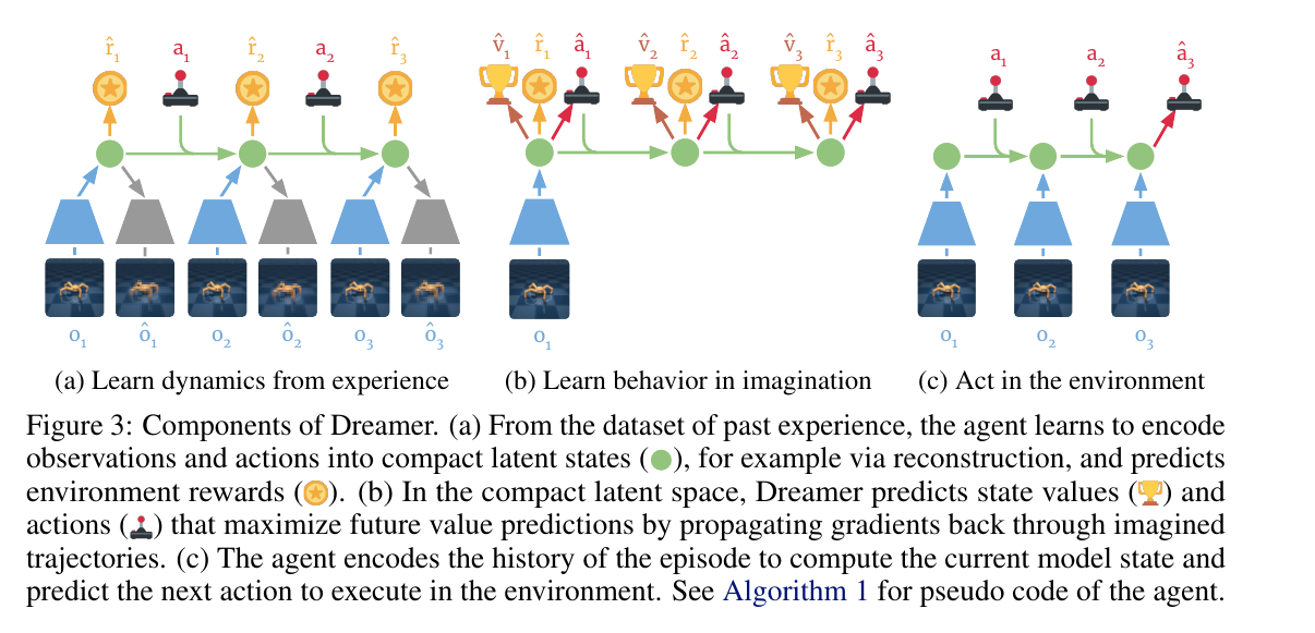
Dreamer: Training a Control Policy in Imagination

The Dreamer series combines world models, latent-space representations, and actor-critic training^[10:1][11:1]. The agent first learns latent dynamics from real interaction, then rolls out many imagined trajectories in latent space and trains the policy on those trajectories.

The importance of DreamerV3 lies in its generality: the same algorithm and hyperparameters achieve strong performance across visual control, continuous control, Atari, Minecraft, and other domains^[11:2]. This moves MBRL from a "sample-efficiency trick" toward a general agent-training framework.

Dreamer's RSSM (Recurrent State-Space Model) divides the latent state into deterministic memory $h_t$ and stochastic variable $z_t$:

$$h_t=f_\phi(h_{t-1}, z_{t-1}, a_{t-1}),\qquad z_t\sim q_\phi(z_t\mid h_t,o_t)$$

You can understand $h_t$ as "the memory so far," and $z_t$ as "the remaining uncertain factors at the current step." $h_t$ updates from the previous memory, stochastic state, and action; $z_t$ combines the current observation $o_t$ to write what was actually seen into the latent state.

The world model simultaneously predicts observations, rewards, and continuation probability:

$$\mathcal{L}_{\text{world}} =\sum_t \left[ -\log p_\phi(o_t\mid h_t,z_t) -\log p_\phi(r_t\mid h_t,z_t) -\log p_\phi(c_t\mid h_t,z_t) +\beta\,\mathrm{KL}\big(q_\phi(z_t\mid h_t,o_t)\,\|\,p_\phi(z_t\mid h_t)\big) \right]$$

This world-model loss has four parts:

Term	What it trains
$-\log p_\phi(o_t\mid h_t,z_t)$	Whether the latent state can explain the current observation
$-\log p_\phi(r_t\mid h_t,z_t)$	Whether the latent state can predict reward
$-\log p_\phi(c_t\mid h_t,z_t)$	Whether the latent state can predict whether the episode continues
$\mathrm{KL}(q_\phi|p_\phi)$	Keeps the posterior state with observation close to the prior state predicted only by the model

The first three terms ask whether "this latent state is useful enough." The KL term prevents the model from working only when it sees real observations, but collapsing during imagined rollout.

After the world model is trained, the actor does not need to access the real environment at every step. It maximizes imagined return inside the model:

$$J(\psi)= \mathbb{E}_{\hat{p}_\phi,\pi_\psi} \left[ \sum_{t=0}^{H}\gamma^t \hat{r}_t \right]$$

This formula resembles the earlier RL objective, but the data source has changed. The reward in the real environment is $r_t$; the reward in Dreamer's imagined trajectory is $\hat{r}_t$. Real environment transitions come from the physical world; Dreamer's transitions come from the learned latent-space world model $\hat{p}_\phi$. The actor parameters are $\psi$, and the training objective is to increase the average imagined return.

Figure 7: Dreamer's latent-imagination training structure. Source: Hafner et al., "Dream to Control", Fig. 3[^dreamer].

Algorithm / series	World model type	Planning or training method	Typical scenario
Dyna	Tabular or function-approximation dynamics model	Use the model to generate experience and update the value function	Classic RL, teaching paradigm
PETS	Probabilistic dynamics model ensemble	MPC + trajectory sampling	Low-sample continuous control
AlphaZero	Known environment rules	MCTS + neural-network evaluation	Go, chess, shogi
MuZero	Learned implicit latent-space model	Latent MCTS	Board games, Atari
Dreamer	Latent RSSM world model	Latent-imagination training	Visual control, robotics, games
TD-MPC2	Task-conditioned latent dynamics model	Latent MPC + policy learning	Large-scale continuous control, multitask settings

Why Embodied Intelligence Especially Needs MBRL

Embodied intelligence and MBRL naturally fit together, not because "MBRL is more advanced," but because the physical world is too expensive, too slow, and too dangerous.

Figure 8: A survey of autonomous-driving world models places physical-world prediction, behavior planning, training data, and application tasks in one structural diagram. Source: Feng et al., "A Survey of World Models for Autonomous Driving", Fig. 1[^adwmsurvey].

1. Real interaction is expensive: collecting one real robot trajectory takes time, and failure may damage hardware. MBRL can move part of exploration into the model.
2. Safety constraints are stronger: filtering out dangerous actions inside the model is safer than letting the real robot discover them through trial and error.
3. Tasks require future prediction: grasping, walking, and obstacle avoidance all depend on short-term dynamics prediction. The consequence of an action is often not visible from the current state alone.
4. Sim-to-real needs uncertainty: probabilistic models and model ensembles can estimate "how uncertain I am," which is especially important when transferring to the real world.

MBRL Is Not a Free Lunch

The core risk of MBRL is model bias: if the world model is wrong, planning will exploit that error, and the policy may learn increasingly biased behavior inside that error. PETS uses probabilistic model ensembles to express uncertainty^[4:1], and Dreamer learns compact dynamics in latent space^[10:2]. In essence, both are trying to control the impact of model error.

Why MBRL Is Mentioned Less Often in Large-Model RL

Chapters 8 to 10 of this book discussed DPO, PPO, GRPO, and Agentic RL, but rarely emphasized MBRL separately. This is not because MBRL is unimportant, but because the language model itself already behaves like a language world model.

When an LLM performs mathematical reasoning or multi-step tool use, it predicts subsequent text, tool results, and intermediate states in token space. Chain of thought can be seen as a kind of internal planning, while search and self-correction can also be seen as "trying a few steps ahead" in language space. Therefore, the LLM field more often says test-time search, self-play, or process reward, rather than dynamics model in the traditional robotics sense.

But the physical world is different. A robot cannot understand friction, contact, latency, and torque from text knowledge alone. It must learn from real or simulated interaction how actions change the world. This is why MBRL becomes crucial again in embodied intelligence.

Relationship to Video World Models

Recent video generation models make one question concrete again: can a video model serve as a robot's world model?

The idea is attractive: given the current image and action, the model generates a video of the next few seconds; the robot chooses the safest and most goal-aligned future among the candidates. OpenAI's Sora technical report also describes large-scale video generation models as a path toward understanding and simulating the physical world^[13].

However, directly using video generation for control still faces several hard problems:

• Insufficient action conditioning: a video model may know "how the picture changes," but not necessarily "what happens after the robot applies a certain torque."
• Insufficient physical consistency: a generated video may look plausible while violating contact, mass conservation, or joint constraints.
• Closed-loop control is difficult: robot control needs feedback at tens to thousands of Hz; video generation models are usually too slow.
• Reward alignment is unclear: a visually pleasing future video is not the same as an executable and safely reachable future state.

Therefore, the more realistic direction is not "directly use a video model to control a robot," but to use video models as part of representation learning, data generation, short-term prediction, or simulation augmentation, and then combine them with RL, MPC, and robot controllers.

Paper Reading: What Problems Do the Representative Works Solve?

Read surveys first, then algorithm papers. If you want to build the map quickly, start with three kinds of surveys: Ding et al.'s general survey is useful for separating the two main threads of "world understanding" and "future prediction"^[1:1]; Li et al.'s embodied AI survey is useful for seeing the taxonomy across function, temporal modeling, and spatial representation^[2:1]; Feng et al.'s autonomous-driving survey helps explain how world models combine perception, prediction, and planning into one engineering loop^[3:1]. The algorithm papers below can be understood as key nodes on this map.

PETS: solving the "low-sample control" problem. The PETS title includes the phrase "in a handful of trials." Its focus is not to propose a bigger neural network, but to combine probabilistic dynamics, model ensembles, and trajectory sampling^[4:2]. When data is scarce, model uncertainty is more important than the model mean; the planner must know which futures are trustworthy and which are only guesses by the model.

MBPO: solving the problem of "when to trust your model." The core of MBPO is not generating model data without limit, but theoretically and experimentally showing that short model rollouts are more reliable^[5:2]. Imagining 1 to 5 steps from real states is often more stable than letting the model roll forward by itself for a long time. This is especially important for robots, because once contact error deviates, later predictions can quickly become distorted.

PlaNet and Dreamer: solving the problem that "pixels are too hard to predict." PlaNet shows that latent-space dynamics can be learned from pixels and used for planning^[9:1]; Dreamer further uses imagined trajectories for actor-critic training^[10:3]. Their shared idea is that control does not require complete reconstruction of future images. It only needs a latent state sufficient to predict rewards and action consequences.

MuZero: solving the problem that "the model need not look like the environment." MuZero's model serves search, not image reconstruction^[8:2]. As long as latent dynamics can predict reward, value, and policy priors, it can support MCTS. This is close to task-oriented world models in embodied intelligence: a robot may not need to generate every pixel; it only needs to know "will this action knock over the cup?"

TD-MPC2: solving the problem of "how to scale continuous control." TD-MPC2 extends latent model predictive control to more tasks and larger models, emphasizing decoder-free task-relevant latent representations^[12:1]. This route is practical for embodied intelligence: instead of spending model capacity reconstructing visual details, concentrate capacity on value, reward, and controllable dynamics.

Reflection question: Will MBRL completely replace model-free RL?

Not in the short term. MBRL has higher sample efficiency, but also higher engineering complexity, and model error introduces additional risk. Model-free methods such as PPO and SAC remain main workhorses in embodied RL, especially in massively parallel simulators like Isaac Lab, where enormous sampling can directly compensate for lower sample efficiency.

The more likely path is hybridization: use model-free methods for stable optimization, and use world models to improve sample efficiency, perform safety filtering, generate imagined trajectories, or assist planning. Modern Dreamer, TD-MPC2, and MuZero are not "pure model" systems. They combine models, policies, value functions, and search.

Connections to Previous Chapters

Concept from earlier chapters	Correspondence in MBRL
MDP transition probability (Chapter 3)	The world model predicts next state, reward, and termination probability
DQN and value functions (Chapter 4)	Dyna uses model-generated experience to update value functions
Policy gradients and actor-critic (Chapters 5-6)	Dreamer trains actor and critic on imagined trajectories
Stable PPO training (Chapter 7)	Embodied RL often uses PPO first to obtain a strong simulation baseline
Embodied intelligence (main article in this section)	MBRL addresses expensive real interaction and the need to predict the future
Offline RL (Section 12.5)	Offline data can be used to pretrain world models before planning or policy optimization

Common Questions

Q1: Can the Environment Simulated by a World Model Be Wrong?

Yes, and this is exactly the core difficulty of MBRL. A world model is not the physical world itself. It is an approximation learned from finite data:

$$\hat{p}_\phi(s_{t+1}, r_t, d_t\mid s_t,a_t)\approx p(s_{t+1}, r_t, d_t\mid s_t,a_t)$$

The left side is the learned world model, and the right side is the real environment. The $\approx$ here does not mean "exactly equal"; it means "we hope it is as close as possible." In reality, data is limited, sensors are noisy, and contact dynamics are complex, so the world model almost certainly contains errors.

As long as $\hat{p}_\phi \neq p$, model rollouts are biased. There are usually three kinds of bias:

1. One-step prediction error: the model predicts $s_{t+1}$, $r_t$, or termination probability inaccurately.
2. Error accumulation: the predicted $\hat{s}_{t+1}$ becomes the input for the next step, so errors are amplified along the rollout.
3. Model exploitation: the planner actively searches for action sequences where the model is overly optimistic. This is called model exploitation.

Mathematically, if total variation distance is used as a rough measure of one-step model error:

$$\epsilon_m = \max_{s,a} D_{\mathrm{TV}}\left( p(\cdot\mid s,a), \hat{p}_\phi(\cdot\mid s,a) \right)$$

You can first understand $D_{\mathrm{TV}}$ as "how different two probability distributions are." $\epsilon_m$ takes the maximum difference over all states and actions, asking: how wrong can the world model be in the worst one-step case?

Then long-horizon value error does not appear only linearly with $\epsilon_m$. It is amplified by the discount factor and planning horizon. A common intuitive form is:

$$\left|V_p^\pi(s)-V_{\hat{p}}^\pi(s)\right| \lesssim \mathcal{O}\left( \frac{\gamma R_{\max}}{(1-\gamma)^2}\epsilon_m \right)$$

The point of this formula is not the constant, but the denominator $(1-\gamma)^2$. The closer $\gamma$ is to 1, the more the agent values the long-term future, the smaller the denominator becomes, and the greater the risk of error amplification. In other words, the longer the planning horizon and the more we trust future return, the larger the value bias caused by a small model error may become.

This is not a theorem to memorize, but an engineering fact to remember: a model error that looks small for one step can become a large value bias in long-horizon planning. The MBPO paper is titled "When to Trust Your Model," and its core conclusion is that model-generated data is convenient but biased, so short rollouts branched from real states should be used^[5:3]. PETS uses probabilistic model ensembles to express uncertainty and avoid blindly trusting a single model^[4:3].

In code, common approaches penalize return when model uncertainty is high, or stop imagination early:

@torch.no_grad()
def conservative_model_step(ensemble, state, action, beta=2.0, stop_threshold=0.5):
    preds = torch.stack([model.sample(state, action) for model in ensemble])
    mean_pred = preds.mean(dim=0)
    uncertainty = preds.var(dim=0).mean(dim=-1)

    delta_state, reward = mean_pred[:, :-1], mean_pred[:, -1]
    reward = reward - beta * uncertainty

    should_stop = uncertainty > stop_threshold
    next_state = state + delta_state
    return next_state, reward, should_stop

So the answer is not simply "whether the world model will be wrong," but "when it is wrong, whether the system can know it is uncertain and pass that uncertainty to the planner." Successful MBRL engineering usually does exactly this: short rollouts, model ensembles, uncertainty penalties, feeding real data back in, and replanning at every step.

Q2: Is the Computational Cost of a World Model Large?

It does add cost, but the question is what you are trading for what. The main cost of model-free methods is environment interaction plus policy/value updates; MBRL adds two more cost components:

$$\text{MBRL cost} \approx \text{model training} + \text{planning or imagination rollout} + \text{policy/value update}$$

This is not a strict formula, but an engineering ledger. Model-free methods usually spend most of their budget on environment sampling and policy updates; MBRL must additionally train the world model and may perform planning or imagined rollout before each decision.

If every decision uses CEM/MPC planning, the computational complexity is roughly:

$$\mathcal{O}(I\cdot N\cdot H\cdot M\cdot C_{\text{model}})$$

Read this expression directly as multiplication: CEM runs for $I$ iterations; each iteration evaluates $N$ candidate action sequences; each sequence looks ahead $H$ steps; if there are $M$ model members, multiple models must run at every step; $C_{\text{model}}$ is the cost of one model forward pass. This overhead cannot be ignored on real-time robots.

What MBRL usually buys in return is fewer real interactions. PETS reaches near-competitive performance on some continuous-control benchmarks with far fewer environment samples than SAC/PPO^[4:4]. Dreamer improves data efficiency, computation time, and final performance on visual-control tasks through latent imagination training^[10:4]. TD-MPC2 further emphasizes decoder-free latent-space world models, doing planning in compact latent space^[12:2].

In engineering terms, the choice can be judged as follows:

Scenario	More suitable choice
Simulation is extremely cheap and massively parallel sampling is easy	Strong model-free baselines such as PPO and SAC
Real interaction is expensive or risky	MBRL, MPC, safety filtering, offline pretraining
Visual inputs are high-dimensional	Latent-space MBRL, such as Dreamer and TD-MPC
Real-time control frequency is very high	Small models, short horizons, policy distillation

A common deployment pattern is: use the world model during training to improve sample efficiency, but do not necessarily perform expensive planning at every deployment step. Instead, distill planning results into a fast policy:

# During training: MPC provides high-quality actions
expert_action = cem_plan(world_model, state, action_dim)

# During distillation: train a fast policy to imitate MPC
policy_action = actor(state)
distill_loss = ((policy_action - expert_action) ** 2).mean()

This is why we should not only ask "is the world model expensive?" We should also ask "how expensive is real-world sampling?" If real interaction is cheap, model-free may be more economical; if real interaction requires hardware, humans, and safety approval, the GPU cost of a world model may be cheaper.

Q3: How Is LeCun's World Model Different from the World Model in MBRL?

LeCun's "world model" is more like a core module in a general agent architecture than a specific RL algorithm. In his 2022 position paper, LeCun argues that agents need configurable predictive world models, intrinsic cost functions, and hierarchical JEPA/H-JEPA representations for self-supervised learning, reasoning, and planning^[14].

The world model in MBRL is usually written as:

$$\hat{p}_\phi(s_{t+1}, r_t, d_t\mid s_t,a_t)$$

It serves control: given a state and action, predict the next state, reward, and termination. PETS, MBPO, Dreamer, and MuZero all fall within this broad category, but their prediction targets differ: PETS predicts low-dimensional state differences, Dreamer predicts latent states and rewards, and MuZero only predicts rewards, values, and policy priors useful for search.

The LeCun/J(EPA) route emphasizes prediction in representation space, rather than generating pixels or directly predicting rewards. I-JEPA predicts target-block representations from image context blocks, without relying on hand-crafted data augmentation or pixel-level reconstruction^[15]. V-JEPA extends this idea to video, with the training objective of predicting video features rather than using text, negative samples, or pixel reconstruction as supervision^[16].

We can place several kinds of "world model" side by side:

Route	What it predicts	Main goal
Classic MBRL	Next state, reward, termination probability	Control, planning, sample efficiency
Video-generation world models	Future pixels or video clips	Generation, simulation augmentation, representation learning
LeCun/J(EPA) route	Abstract representations, future embeddings	Self-supervised representation, common sense, hierarchical planning
MuZero/Dreamer style	Latent states, rewards, values, or policy-relevant information	Learn only the model useful for decision-making

The core JEPA form can be written as:

$$z_y = E_{\bar{\theta}}(y),\qquad \hat{z}_y = P_\phi(E_\theta(x), c),\qquad \mathcal{L}_{\text{JEPA}} = \|\hat{z}_y-\mathrm{sg}(z_y)\|_2^2+\Omega(z)$$

Read this formula as follows: first, the target encoder $E_{\bar{\theta}}$ encodes the target region $y$ into representation $z_y$; then the context encoder $E_\theta$ sees the visible region $x$, and the predictor $P_\phi$ guesses the target representation $\hat{z}_y$; the loss makes the predicted representation close to the true target representation. $\mathrm{sg}$ means stop-gradient: the target side is treated as the answer, and gradients are not allowed to change the answer itself.

Figure 9: Video-JEPA's joint-embedding predictive architecture predicts target video-segment embeddings in representation space. Source: Bardes et al., "Revisiting Feature Prediction for Learning Visual Representations from Video", Fig. 2[^vjepa].

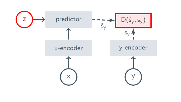
Here, $x$ is the visible context, $y$ is the masked or future target, $c$ may contain position, time, or action conditions, $\mathrm{sg}$ denotes stop-gradient, and $\Omega$ is a regularizer that prevents representation collapse. Compared with pixel generation, it does not require the model to recover every texture detail. Compared with traditional MBRL, it also does not necessarily output reward directly. The 2026 LeWorldModel further trains JEPA from raw pixels into an end-to-end world model usable for control, which is a recent example of this route moving closer to embodied control^[17].

In one sentence: MBRL world models lean toward "control engineering," while LeCun's world model leans toward "general intelligence architecture"; the former asks how the world changes after an action, while the latter asks how an agent can learn abstract world representations that are predictable and plannable.

Q4: What Is the Mathematical Difference Between Model-Based and Model-Free?

Both optimize the same RL objective:

$$J(\theta) = \mathbb{E}_{\tau\sim p,\pi_\theta} \left[ \sum_{t=0}^{\infty}\gamma^t r_t \right]$$

That is, both model-free and model-based methods ultimately want the policy to obtain higher long-term return. The difference is not "whether the goal is reward maximization," but where the next states and future returns come from when updating this objective.

The difference is whether $p(s_{t+1},r_t\mid s_t,a_t)$ is explicitly learned.

Model-Free does not model environment transitions. It directly uses sampled $(s,a,r,s')$ from the real environment or simulator to update the policy or value function. For example, the critic target in Q-learning / SAC style is:

$$y_t = r_t+\gamma(1-d_t)Q_{\bar{\theta}}(s_{t+1}, \pi_\psi(s_{t+1}))$$

Here, $s_{t+1}$ comes from the real replay buffer, not from model prediction. The critic uses a one-step transition that actually happened to construct the answer $y_t$.

Model-Based first learns a model:

$$\mathcal{L}_{\text{model}}(\phi) = -\mathbb{E}_{\mathcal{D}} \log \hat{p}_\phi(s_{t+1}, r_t, d_t\mid s_t,a_t)$$

This loss means that the world model should assign higher probability to the next states, rewards, and termination flags that really occurred. The negative sign comes from maximum-likelihood training: we want to maximize the probability of real data, but optimizers usually minimize a loss, so we write negative log likelihood.

Then the model is used for planning:

$$a_{0:H-1}^{*} = \arg\max_{a_{0:H-1}} \sum_{h=0}^{H-1} \gamma^h \hat{r}_\phi(\hat{s}_{t+h}, a_{t+h})$$

Here, both $\hat{s}$ and $\hat{r}$ are imagined by the model. The planner does not need to try every action sequence in the real environment; it scores them first inside the world model.

Or the imagined trajectories can be used to train the policy:

$$J_{\text{imag}}(\psi) = \mathbb{E}_{\hat{p}_\phi,\pi_\psi} \left[ \sum_{h=0}^{H} \gamma^h \hat{r}_{t+h} \right]$$

This $J_{\text{imag}}$ looks much like the real RL objective, but its trajectories come from $\hat{p}_\phi$, not from the real environment $p$. Therefore, the mathematical difference is not "different objective," but where the gradients and data come from. Model-free learning signals mainly come from real samples; model-based methods add a differentiable or sampleable world model, so learning signals can also come from model rollouts.

Q5: What Does the Code Difference Between Model-Based and Model-Free Look Like?

First look at model-free. There is no world_model here; next_state is the next state that actually appeared in the replay buffer:

# Model-Free: SAC / DDPG-style critic update
state, action, reward, next_state, done = replay.sample()

with torch.no_grad():
    next_action = actor(next_state)
    target_q = target_critic(next_state, next_action)
    y = reward + gamma * (1.0 - done) * target_q

q = critic(state, action)
critic_loss = ((q - y) ** 2).mean()
critic_loss.backward()
critic_optimizer.step()

Now look at model-based. The code adds a model-training step, plus a planning or imagination step that predicts the future with the model:

# Model-Based: first train the world model
state, action, reward, next_state, done = replay.sample()
target = torch.cat([next_state - state, reward, done], dim=-1)

mu, logvar = world_model(state, action)
model_loss = gaussian_nll(mu, logvar, target)
model_loss.backward()
model_optimizer.step()

# Then use the world model to generate imagined transitions
imagined_state = state
imagined_return = 0.0
discount = 1.0

for h in range(horizon):
    imagined_action = actor(imagined_state)
    pred = world_model.sample(imagined_state, imagined_action)
    delta_state, imagined_reward, imagined_done = split_prediction(pred)

    imagined_return += discount * imagined_reward
    discount *= gamma * (1.0 - imagined_done)
    imagined_state = imagined_state + delta_state

actor_loss = -imagined_return.mean()
actor_loss.backward()
actor_optimizer.step()

This comparison shows the essential engineering difference:

• In model-free code, next_state is provided by the dataset.
• In model-based code, imagined_state is rolled out by the model.
• Model-free code is shorter, more stable, and more dependent on sampling.
• Model-based code is more complex and saves real interaction, but must handle model error.

Q6: Can a World Model Replace a Real Simulator?

In the short term, not completely. A physical simulator such as MuJoCo or Isaac Sim is a hand-written approximate physics engine. A world model is a statistical approximation learned from data. The former has explicit geometry, joints, collisions, and integrators; the latter has stronger data adaptation, but is more likely to fail in out-of-distribution states.

The more practical relationship is complementary:

1. The simulator generates data: use large-scale simulated trajectories to pretrain the world model.
2. The world model provides a fast approximation: short-term planning in latent space can be cheaper than high-fidelity simulation.
3. Real robot data corrects the model: use real interaction for residual dynamics or domain adaptation.
4. Safety filtering: the world model filters obviously dangerous actions before passing control to a low-level controller.

MuZero's experience also shows that a model does not necessarily need to reconstruct the full environment. It only needs to predict information useful for planning in order to support strong search^[8:3]. This matters for robotics, because "completely simulating the world" is too hard, while "predicting whether the cup will be pushed over, the foot will slip, or the gripper will collide" is closer to a solvable problem.

Q7: When Should We Prefer MBRL, and When Should We Continue Using Model-Free?

Use a simple judgment:

Prefer MBRL when real interaction is expensive, failures are costly, short-term prediction is needed, offline data should be reused, the task is sensitive to safety constraints, or the state has clear dynamics structure. Robotic grasping, legged locomotion, autonomous-driving boundary scenarios, and real laboratory control all fall into this category.

Prefer model-free when the simulation environment is cheap, rewards are clear, parallel sampling is easy, and engineering needs a stable baseline. PPO remains very strong in parallel simulators such as Isaac Lab, because massive simulated steps can offset lower sample efficiency.

The most common modern route is hybrid: first obtain a stable policy with model-free methods, then use a world model to improve sample efficiency, perform safety filtering, generate short imagined trajectories, or correct policy actions with MPC during deployment. Representative algorithms such as Dreamer, TD-MPC2, and MuZero are not "pure model" or "pure policy" methods. They combine models, policies, value functions, and planning.

Q8: Why Use PETS Here? Should Beginners Implement PETS Directly?

PETS is cited here because the paper places several key MBRL components into one interpretable framework: dynamics models, model uncertainty, trajectory propagation, and MPC^[4:5]. It is especially suitable for answering questions such as "will the model learn incorrectly?" and "why can the planner not blindly trust the model?"

But beginners should not start by directly implementing PETS. A better sequence is:

1. First implement a deterministic world model: $f_\phi(s_t,a_t)\rightarrow[\Delta s_t,r_t]$.
2. Then implement random-shooting MPC: sample action sequences, predict returns with the model, and execute the first action.
3. After confirming that the closed loop works, replace the single model with a probabilistic model or model ensemble.

Mathematically, the minimal version only learns a point estimate:

$$\widehat{\Delta s_t},\hat r_t=f_\phi(s_t,a_t)$$

PETS turns prediction into a distribution and uses multiple model members to represent epistemic uncertainty:

$$p_{\phi_i}(\Delta s_t,r_t\mid s_t,a_t) =\mathcal{N}(\mu_{\phi_i},\Sigma_{\phi_i})$$

In code, the minimal version is one network plus MSE loss. PETS uses multiple probabilistic networks plus Gaussian NLL, and performs sampling propagation for future trajectories during planning. The former is suitable for learning the skeleton of MBRL; the latter is suitable for the more common real-robot situation where data is scarce, noise is large, and contact is uncertain.

Summary

Model-free RL learns "what to do." Model-based RL also learns "what will happen to the world after doing this." In digital environments where interaction is cheap, model-free methods are often direct enough. In physical tasks such as robotics, autonomous driving, and complex manipulation, world models can significantly reduce trial-and-error cost and provide leverage for planning, safety constraints, and generalization.

The difficulty of MBRL is also clear: models cannot be perfect, and model error can be amplified by planning. Truly effective systems usually do not choose between model-free and model-based as mutually exclusive options. They place world models, policy learning, search planning, and real feedback into one closed loop.

As a next step, return to the main embodied intelligence article and connect the world-model perspective here with sim-to-real, domain randomization, and VLA models.

---

References:

---

1. Ding, J. et al. (2025). Understanding World or Predicting Future? A Comprehensive Survey of World Models. ACM Computing Surveys. https://arxiv.org/abs/2411.14499 ↩︎ ↩︎

2. Li, X. et al. (2025). A Comprehensive Survey on World Models for Embodied AI. https://arxiv.org/abs/2510.16732 ↩︎ ↩︎

3. Feng, T. et al. (2025). A Survey of World Models for Autonomous Driving. https://arxiv.org/abs/2501.11260 ↩︎ ↩︎

4. Chua, K. et al. (2018). Deep Reinforcement Learning in a Handful of Trials using Probabilistic Dynamics Models. NeurIPS. https://arxiv.org/abs/1805.12114 ↩︎ ↩︎ ↩︎ ↩︎ ↩︎ ↩︎

5. Janner, M. et al. (2019). When to Trust Your Model: Model-Based Policy Optimization. NeurIPS. https://arxiv.org/abs/1906.08253 ↩︎ ↩︎ ↩︎ ↩︎

6. Sutton, R. S. (1991). Dyna, an Integrated Architecture for Learning, Planning, and Reacting. SIGART Bulletin. https://www.incompleteideas.net/papers/sutton-91dyna.pdf ↩︎

7. Silver, D. et al. (2017). Mastering Chess and Shogi by Self-Play with a General Reinforcement Learning Algorithm. https://arxiv.org/abs/1712.01815 ↩︎ ↩︎

8. Schrittwieser, J. et al. (2020). Mastering Atari, Go, Chess and Shogi by Planning with a Learned Model. Nature. https://arxiv.org/abs/1911.08265 ↩︎ ↩︎ ↩︎ ↩︎

9. Hafner, D. et al. (2019). Learning Latent Dynamics for Planning from Pixels. ICML. https://arxiv.org/abs/1811.04551 ↩︎ ↩︎

10. Hafner, D. et al. (2020). Dream to Control: Learning Behaviors by Latent Imagination. ICLR. https://arxiv.org/abs/1912.01603 ↩︎ ↩︎ ↩︎ ↩︎ ↩︎

11. Hafner, D. et al. (2023). Mastering Diverse Domains through World Models. https://arxiv.org/abs/2301.04104 ↩︎ ↩︎ ↩︎

12. Hansen, N. et al. (2024). TD-MPC2: Scalable, Robust World Models for Continuous Control. ICLR. https://arxiv.org/abs/2310.16828 ↩︎ ↩︎ ↩︎

13. Brooks, T. et al. (2024). Video generation models as world simulators. OpenAI. https://openai.com/index/video-generation-models-as-world-simulators/ ↩︎

14. LeCun, Y. (2022). A Path Towards Autonomous Machine Intelligence. OpenReview. https://openreview.net/forum?id=BZ5a1r-kVsf ↩︎

15. Assran, M. et al. (2023). Self-Supervised Learning from Images with a Joint-Embedding Predictive Architecture. CVPR. https://arxiv.org/abs/2301.08243 ↩︎

16. Bardes, A. et al. (2024). Revisiting Feature Prediction for Learning Visual Representations from Video. https://arxiv.org/abs/2404.08471 ↩︎

17. Maes, J. et al. (2026). LeWorldModel: A Unified End-to-End World Model for Autonomous Driving. https://arxiv.org/abs/2603.19312 ↩︎