3.6 From Value to Policy

What This Section Solves

Core content

• Limits of value-based RL: $\arg\max_a Q(s,a)$ is not directly solvable in continuous or extremely large action spaces.
• Parameterized policies: model behavior directly with $\pi_\theta(a \mid s)$ instead of an explicit $Q$ table.
• Policy objective and gradients: define $J(\theta)$ as the policy's expected return; the policy gradient theorem gives an optimization direction.
• REINFORCE and variance: update from trajectory returns, but variance is high and baselines are needed for stability.

The previous section focused on value-based reinforcement learning: we store an estimate $Q(s,a)$ for each state-action pair, and derive a policy by

$$a = \arg\max_a Q(s,a).$$

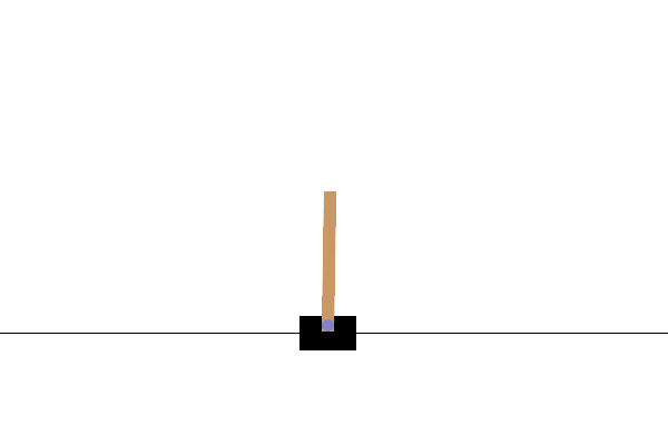
This works well when the action space is small. In CartPole there are only two actions (push left / push right), so comparing $Q$ values is easy.

But the key operation above hides an assumption:

actions must be enumerable.

Once the action space becomes continuous or too large, this assumption breaks. A robot arm might output torques for 6 joints:

$$a=(\tau_1,\tau_2,\ldots,\tau_6)\in\mathbb{R}^6.$$

You can train a network $Q(s,a)$ that scores actions, but the real difficulty comes next: how do you solve

$$\arg\max_a Q(s,a)$$

over infinitely many $a$?

In autonomous driving, throttle and steering are continuous. In language modeling, the action space is a vocabulary with tens of thousands of tokens. In these settings, “score every action then take the maximum” becomes computationally and algorithmically awkward.

So if what we ultimately need is an agent that acts, why insist on learning a score table first?

The core idea is:

model the policy directly.

Instead of deriving behavior indirectly from a value function, we let a policy network output an action distribution (or a continuous action) and optimize its parameters using the return signal from the environment. This is the policy-based route.

Core concept

There are two common routes in RL.

Value-based methods learn action values $Q(s,a)$ and choose actions via $\arg\max_a Q(s,a)$ (Q-learning, DQN). They are a natural fit when actions are few and comparable, and they often reuse old data efficiently via replay buffers.

Policy-based methods learn a policy $\pi_\theta(a\mid s)$ directly: the probability of choosing action $a$ in state $s$ (REINFORCE and policy gradients). They optimize the policy's expected return:

$$J(\theta)=\mathbb{E}_{\tau\sim\pi_\theta}[G_0].$$

Intuitively, actions that occur in high-return trajectories increase in probability, and actions in low-return trajectories decrease. Because the policy outputs a distribution (or continuous actions) directly, this route is well-suited to robotics, autonomous driving, and LLM generation. Pure policy gradients are often more on-policy because they rely on fresh samples from the current policy. ^[1][^5][^6]

From Action Scores to a Behavior Distribution

In value-based RL, we estimate $Q(s,a)$ and choose the larger value.

Now consider a different representation. Instead of asking “which action has the highest score?”, we model how the agent behaves: what distribution over actions does it follow in state $s$?

For example, a policy might specify: in state $s$, push left with probability 70% and push right with probability 30%. In environments with more actions, the policy is a full distribution across all choices.

Early in training, this distribution is usually wrong. The agent interacts with the environment using the current distribution, receives returns, and adjusts the distribution:

• actions that frequently appear in high-return trajectories should become more probable in the corresponding states;
• actions that frequently appear in low-return trajectories should become less probable.

So the policy route shifts the question: from “which action scores highest” to “how should I act”.

Parameterized Policies

To learn from data, we introduce parameters into the policy:

$$\pi_\theta(a\mid s)=P_\theta(A_t=a\mid S_t=s).$$

Here $\theta$ are the learnable parameters (typically neural network weights). $S_t$ is the state and $A_t$ is the chosen action at time $t$.

For discrete action spaces, the network often outputs a preference score (logit) $z_\theta(s,a)$ for each action. We convert logits into a valid probability distribution using softmax:

$$\pi_\theta(a\mid s) = \frac{\exp(z_\theta(s,a))} {\sum_{a'}\exp(z_\theta(s,a'))}.$$

For continuous control, we cannot enumerate actions, so a common choice is to represent the policy as a continuous distribution, such as a Gaussian:

$$a\sim\mathcal{N}\left(\mu_\theta(s),\sigma_\theta(s)^2\right).$$

The network outputs $\mu_\theta(s)$ and $\sigma_\theta(s)$: the mean encodes the most likely action and the standard deviation controls stochasticity (and thus exploration).

Note the difference in what $Q$ and $\pi_\theta$ represent:

$$Q(s,a)\quad\text{vs.}\quad \pi_\theta(a\mid s).$$

$Q(s,a)$ evaluates the long-term value of taking action $a$ in state $s$. $\pi_\theta(a\mid s)$ defines the probability of choosing $a$ in $s$.

The Policy Objective $J(\theta)$

Once we have a parameterized policy, the next question is: are these parameters good?

In value-based RL we compare actions inside a single state. Now we zoom out: we want to evaluate the entire policy.

If initial states are drawn from a distribution $\rho_0$, a standard objective is

$$J(\theta) = \mathbb{E}_{s_0\sim\rho_0} \left[ V^{\pi_\theta}(s_0) \right].$$

Equivalently, in trajectory form, let

$$\tau=(s_0,a_0,r_0,s_1,a_1,r_1,\ldots)$$

and

$$G_0=\sum_{t=0}^{\infty}\gamma^t r_t.$$

Then

$$J(\theta) = \mathbb{E}_{\tau\sim\pi_\theta}[G_0] = \mathbb{E}_{\tau\sim\pi_\theta} \left[ \sum_{t=0}^{\infty}\gamma^t r_t \right].$$

Read it literally:

$$J(\theta)=\text{the expected long-term return achieved by the current policy parameters } \theta.$$

The learning problem becomes a direct optimization problem:

$$\theta^*=\arg\max_\theta J(\theta).$$

Compare this with value-based selection:

• $\arg\max_a Q(s,a)$ chooses an action within a state.
• $\arg\max_\theta J(\theta)$ chooses policy parameters across all behaviors.

Trajectory Probability (Why Policy Gradients Are Subtle)

If we want to optimize $J(\theta)$, the natural next step is to take a gradient:

$$\nabla_\theta J(\theta).$$

But unlike supervised learning, policy optimization does not operate on a fixed dataset. When $\theta$ changes, action probabilities change, which changes visited states, which changes the trajectories we sample.

So it helps to write the probability of a trajectory under parameters $\theta$:

$$P_\theta(\tau) = \rho_0(s_0) \prod_t \pi_\theta(a_t\mid s_t)\, P(s_{t+1}\mid s_t,a_t).$$

Reading left to right:

• $\rho_0(s_0)$ is the probability of the initial state.
• $\pi_\theta(a_t\mid s_t)$ is the policy's action probability.
• $P(s_{t+1}\mid s_t,a_t)$ is the environment transition probability.

Only the policy terms $\pi_\theta(a_t\mid s_t)$ depend on $\theta$; the initial-state distribution and environment dynamics are properties of the environment.

In the next chapter (policy gradients), we will use this structure to derive REINFORCE and the policy gradient theorem, and then discuss variance reduction (baselines and advantage functions).

The Log-Derivative Trick

To optimize the policy objective, write it as a sum over trajectories:

$$J(\theta) = \sum_\tau P_\theta(\tau)G(\tau).$$

Now take a gradient:

$$\nabla_\theta J(\theta) = \sum_\tau \nabla_\theta P_\theta(\tau)G(\tau).$$

Once a trajectory $\tau$ is fixed, its states, actions, and rewards are fixed. The return $G(\tau)$ is treated as a constant with respect to $\theta$. What changes with $\theta$ is the probability of sampling that trajectory.

The expression still contains $\nabla_\theta P_\theta(\tau)$, which is awkward for sampling. We want a form like $P_\theta(\tau)(\cdots)$, because then we can estimate the expectation by drawing trajectories from the current policy.

The key identity is:

$$\nabla_\theta P_\theta(\tau) = P_\theta(\tau)\nabla_\theta\log P_\theta(\tau).$$

It follows from

$$\nabla_\theta\log f(\theta) = \frac{\nabla_\theta f(\theta)}{f(\theta)}.$$

Substituting gives

$$\nabla_\theta J(\theta) = \sum_\tau P_\theta(\tau) \nabla_\theta\log P_\theta(\tau) G(\tau),$$

or equivalently,

$$\nabla_\theta J(\theta) = \mathbb{E}_{\tau\sim\pi_\theta} \left[ \nabla_\theta\log P_\theta(\tau)G(\tau) \right].$$

Now use the trajectory probability from the previous section:

$$\log P_\theta(\tau) = \log \rho_0(s_0) + \sum_t\log\pi_\theta(a_t\mid s_t) + \sum_t\log P(s_{t+1}\mid s_t,a_t).$$

Only the policy terms depend on $\theta$. Therefore,

$$\nabla_\theta\log P_\theta(\tau) = \sum_t\nabla_\theta\log\pi_\theta(a_t\mid s_t).$$

This yields the basic policy gradient form:

$$\nabla_\theta J(\theta) = \mathbb{E}_{\tau\sim\pi_\theta} \left[ \sum_t \nabla_\theta\log\pi_\theta(a_t\mid s_t) G(\tau) \right].$$

Usually, the action at time $t$ should be credited only for rewards that occur after it, so we replace the full trajectory return with the return-to-go:

$$G_t=\sum_{k=t}^{\infty}\gamma^{k-t}r_k.$$

The more common form is therefore

$$\nabla_\theta J(\theta) = \mathbb{E}_{\tau\sim\pi_\theta} \left[ \sum_t \nabla_\theta\log\pi_\theta(a_t\mid s_t) G_t \right].$$

The term $\nabla_\theta\log\pi_\theta(a_t\mid s_t)$ points in the direction that makes the sampled action more likely. The scalar $G_t$ decides how strongly to push in that direction.

The plain-language reading is:

If an action was followed by high return, increase its probability in similar states. If it was followed by low return, decrease it.

A Two-Action Example

Consider a one-state task with two actions, A and B. Let one parameter $\theta$ control the probability of A:

$$p=\pi_\theta(A)=\sigma(\theta), \qquad \pi_\theta(B)=1-p.$$

For this parameterization,

$$\nabla_\theta\log\pi_\theta(A)=1-p,$$

and

$$\nabla_\theta\log\pi_\theta(B)=-p.$$

Suppose $p=0.7$.

If the agent samples A and later receives $G=10$, the update direction is proportional to

$$(1-p)G=0.3\times 10=3.$$

The gradient is positive, so $\theta$ increases and A becomes more probable.

If the agent samples B and later receives $G=10$, the update direction is proportional to

$$(-p)G=-0.7\times 10=-7.$$

The gradient is negative, so $\theta$ decreases, which lowers the probability of A and raises the probability of B.

So policy gradients do not blindly reinforce every action. They reinforce the action that was actually sampled, and the direction depends on the return that followed it.

CartPole and REINFORCE

In CartPole, the state is a 4D vector and the action space has two choices: push left or push right.

REINFORCE applies the policy gradient idea directly:

1. run one full episode using the current policy $\pi_\theta$;
2. record states, actions, log probabilities, and rewards;
3. compute return-to-go $G_t$ for every step;
4. update parameters with

$$\theta \leftarrow \theta + \alpha \sum_t \nabla_\theta\log\pi_\theta(a_t\mid s_t)G_t.$$

A minimal PyTorch implementation has the following structure:

env = gym.make("CartPole-v1")
policy = PolicyNet()
optimizer = torch.optim.Adam(policy.parameters(), lr=1e-2)
gamma = 0.99

for episode in range(500):
    state, _ = env.reset()
    log_probs = []
    rewards = []
    done = False

    while not done:
        action, log_prob = policy.select_action(state)
        next_state, reward, terminated, truncated, _ = env.step(action)
        done = terminated or truncated
        log_probs.append(log_prob)
        rewards.append(reward)
        state = next_state

    returns = []
    G = 0
    for r in reversed(rewards):
        G = r + gamma * G
        returns.insert(0, G)

    returns = torch.tensor(returns, dtype=torch.float32)
    returns = (returns - returns.mean()) / (returns.std() + 1e-8)

    loss = -sum(lp * Gt for lp, Gt in zip(log_probs, returns))
    optimizer.zero_grad()
    loss.backward()
    optimizer.step()

The negative sign appears because PyTorch optimizers minimize losses, while policy gradient is a gradient-ascent method.

Sparse Rewards: Why REINFORCE Can Struggle

CartPole gives a reward at every step, so the policy receives frequent feedback. Many environments are not like this.

MountainCar is a useful contrast: the car starts in a valley and must build momentum to reach the hilltop.

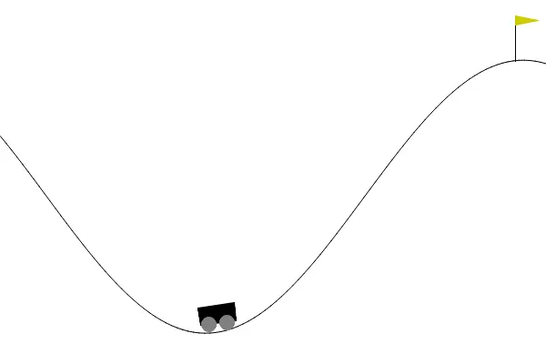
The reward is usually $-1$ per step until success, and a random policy almost never reaches the goal. Then most sampled trajectories look equally bad. If every episode returns roughly $-200$, REINFORCE has little information about which early actions were useful.

This is the sparse-reward problem. TD methods and Q-learning can sometimes propagate value backward from rare successful states more efficiently, while pure Monte Carlo policy gradients must wait for whole-episode returns.

Compared With Q-Learning

The two routes solve different problems well:

Aspect	Q-Learning	REINFORCE
Learns	action values $Q(s,a)$	policy parameters $\theta$
Update timing	every step	after an episode
Data style	often off-policy	on-policy
Action spaces	best for finite discrete actions	works for discrete or continuous policies
Strength	sample reuse and TD propagation	direct policy optimization
Weakness	hard $\arg\max$ in continuous spaces	high variance

They are not enemies. Actor-Critic methods combine them: an Actor learns the policy, while a Critic estimates values to stabilize the policy update.

High Variance and Baselines

Policy gradients can be noisy because returns vary across episodes. In CartPole, one rollout might last 190 steps and another 40 steps under nearly the same policy. Multiplying log-probability gradients by raw returns can make updates unstable.

A more precise question is not:

$$\text{Was the return positive?}$$

but:

$$\text{Was this action better than the usual action in this state?}$$

This leads back to value functions. The state value $V^\pi(s)$ can serve as a baseline: the expected return from state $s$ under the current policy. The advantage function is

$$A^\pi(s,a)=Q^\pi(s,a)-V^\pi(s).$$

If $A^\pi(s,a)>0$, action $a$ is better than average in state $s$ and should become more likely. If $A^\pi(s,a)<0$, it is worse than average and should become less likely.

This is the basic motivation for Actor-Critic:

• the Actor $\pi_\theta$ chooses actions;
• the Critic $V_\phi(s)$ or $Q_\phi(s,a)$ provides a lower-variance learning signal.

REINFORCE uses sampled returns directly. Actor-Critic replaces raw returns with value or advantage estimates. PPO then adds a constraint that prevents each policy update from moving too far.

Relationship to Neighboring Sections

The previous section introduced value-based RL: learn $Q(s,a)$, then act using $\arg\max_a Q(s,a)$. This works naturally when the action space is small and enumerable.

This section introduced policy-based RL: learn $\pi_\theta(a\mid s)$ directly, then optimize expected return $J(\theta)$. This is natural for continuous control, large discrete spaces, and stochastic policies.

The next section asks where the data comes from. Both value updates and policy gradients require trajectories, transitions, or preference data. Whether those data are on-policy, off-policy, online, or offline changes the algorithmic regime.

Summary

1. Value-based methods learn $Q(s,a)$ and choose actions using $\arg\max_a Q(s,a)$.
2. Policy-based methods learn $\pi_\theta(a\mid s)$ directly.
3. The policy objective is $J(\theta)=\mathbb{E}_{\tau\sim\pi_\theta}[G_0]$.
4. The trajectory probability separates policy terms from environment terms.
5. The log-derivative trick turns $\nabla_\theta J(\theta)$ into an expectation that can be estimated from sampled trajectories.
6. REINFORCE is the most direct policy-gradient algorithm, but it has high variance.
7. Baselines, advantages, Actor-Critic, and PPO are progressively more stable ways to use the same objective.

Previous: Action-Value Functions

Next: Data Sources

References

---

1. Williams, R. J. (1992). Simple statistical gradient-following algorithms for connectionist reinforcement learning. Machine Learning, 8, 229-256. ↩︎